Automating Tinder Likes with Support Vector Machine Learning
December 19, 2016
Update
After some careful consideration, the method described here doesn’t work. Instead of focusing on the prediction accuracy for the entire sample, I should actually focus on the Like accruacy for model selection. The reason is that if the number of Dislikes are much greater than the number of Likes then the modeling process will have bias towards Dislikes and be more likely to get would be Likes incorrect. I’ll work more on this and post an update when ready.
Abstract
A support vector machine was used to perform image classification on 8,500 Tinder profiles. Entire profiles were recorded using a custom-built application that used the pynder Python library. Each profile considered has a binary choice, either a Like or a Dislike. The recorded profiles were manually liked or disliked based on the users’s preference. Images were processed into 32 bin histograms, and the bin intensities were used as the variables for the classification problem. Using 10-fold cross validation a support vector machine was selected with an estimated prediction accuracy of 71%. The support vector machine was then introduced to the custom application such that Tinder likes and dislikes can be administered according to the user’s historical preference. The result is a bot capable of automatically liking Tinder profiles, without any user intervention, with an estimated 71% accuracy.
Introduction
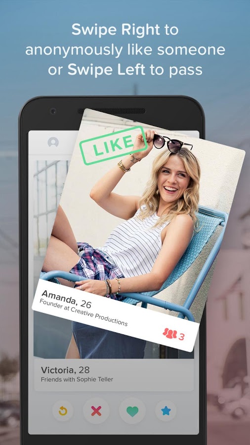
Tinder is the most popular online dating application for mobile devices. Like many other online dating applications, users can set basic preferences (distance, age, gender) for which Tinder profiles they will browse. Profiles are displayed to the user one at a time, containing a cover profile image, name, age, short bio, and mutual friends. The user can choose to view additional images of the profile if desired. The user must either Like or Dislike the profile, at which point the user will be presented with another profile. The process is repeated almost indefinitely. The image below was taken from the Google Play store and demonstrates the Tinder user interface for browsing profiles. When two users Like each other, they will be notified and allowed to message each other if they desire to do so. Tinder is often criticized for it’s shallow online dating selection, and has been demonized as a sex app.
In my opinion Tinder is not a perfect online dating solution. Personally I would like to have access to statistical analysis of the profiles browsed. However my biggest grievance with Tinder is the amount of time required to Like and Dislike profiles. As a busy individual online dating is meant to be a time-friendly solution. However manually browsing profiles, reading short bio’s, and browsing for additional pictures takes a significant amount of time. It feels like such a waste just to Like a user who may not Like you back. It doesn’t appear that Tinder presents you with profiles that you are more likely to Like based on your selection history (and if Tinder is doing so then they are doing a very poor job at it!).
A while ago, I read a very interesting 2015 blog post by Justin Long. Justin described how he created a program to completely automate everything on Tinder. The program uses artificial neural networks and eigenfaces to predict user’s likes or dislikes to a claimed 80% accuracy. I have my personal doubts about the claimed accuracy of Justin’s method. To accurately train the neural networks would require a significantly large database, and obtaining that database would require a significant time contribution from the user. Especially considering the eigenface method may introduce a large number of variables. Though Justin went even one step further and included an auto messaging bot that would automatically send a few messages to a new match. Overall I was extremely impressed with Justin’s work and saved the blog post to reference for a later date.
I knew that If I was to ever use Tinder I would not be a standard user, and I would want to implement some form of automation using machine learning similar to Justin’s work. Additionally with online dating, I would want to perform some sort of statical analysis to determine if my online dating profile and messages were working. With this in mind, I needed to create an application that would record absolutely everything from each Tinder profile I browsed.
There is a Python library called pynder which can be used to access Tinder’s reverse engineered API. I used pynder to create a Python application to Like and Dislike Tinder profiles, recording every detail from each profile during the process. I wanted to get up to 10,000 profiles as I figured the more data I’d have, the better my classification model could be. However I only managed to browse 8,500 profiles before finding a pretty awesome girlfriend along the way. It would take me about 1 hour to go through 100 profiles. So with that estimate I spent 85 hours looking at Tinder profiles (remember I said that Tinder takes up a lot of time), over the course of five or six weeks.
My goal was to automate the Like and Dislike process of Tinder profiles with a machine learning classification model. I wasn’t interested in creating a messaging bot, as I like to come up with a unique first message on Tinder. Image classification has been a popular field in machine learning, with a variety of techniques. I stumbled upon a 1999 article by Chapelle et al. [1] which described a process of using histograms to for support vector machines to perform image classification. As oppose to the eigienface method used by Jason, I thought the histograms would be an easier method to initially work with. Not to mention that it is possible that I would Like a user profile that did not have a picture of a face in it. Additionally I’ve been waiting for an interesting problem to apply support vector machines to.
Support vector machines were used to create an image classification model to Like or Dislike Tinder profiles based on profiles recorded on a custom application. This post details how profile images were processed into 32 bin histograms. The intensity of each bin was used as the variables for the classification problem. Sci-kit learn by Pedregosa et al. [2] is a Python machine learning library which was used to create the support vector classification model. The model was then implemented in the custom appellation to automatically Like or Dislike Tinder profiles with an estimated 71% accuracy.
Image processing
The dataset that was acquired contains Likes and Dislikes for 8,500 Tinder profiles. Each profile has at least one 640x640 px image, with several profiles having multiple 640x640 px images. Thirty-two bin histograms were created for each image in the dataset using Python.
Scipy’s misc.imread was used to read the image files as arrays into Python. For each pixel there is red, green, and blue value that is between 0 and 255. In order to use one histogram, I converted images from RGB to grayscale such that each pixel had a unique value between 0 and 255. Then using NumPy it is easy to create a 32 bin histogram of the image. Why 32 bins? No reason in particular, but I figured it would be a promising starting point. Also it turns out that 32 squared was less than the number of data points in my dataset. I’ve provided some Python code to create the histograms from the collected profile images below.
import numpy as np
from scipy import misc

#	a function to convert a RGB pixel to grayscale
def rgb2gray(rgb):
    return np.dot(rgb[...,:3], [0.299, 0.587, 0.114])

#	histogram bin spacing
binSpacing = np.linspace(0.0, 255, num=33)

#	read the image file
image = misc.imread('TinderProfileImage.jpg')
#	convert the image to grayscale
gray = rgb2gray(image)

#	create a 32 bin histogram
hist = np.histogram(gray,bins=binSpacing)
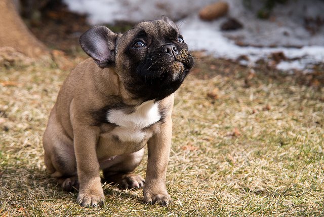
It may not necessary be clear as to what an image looks like as a 32 bin histogram, so I’ve processed this dog image.
 Which becomes the following histogram.
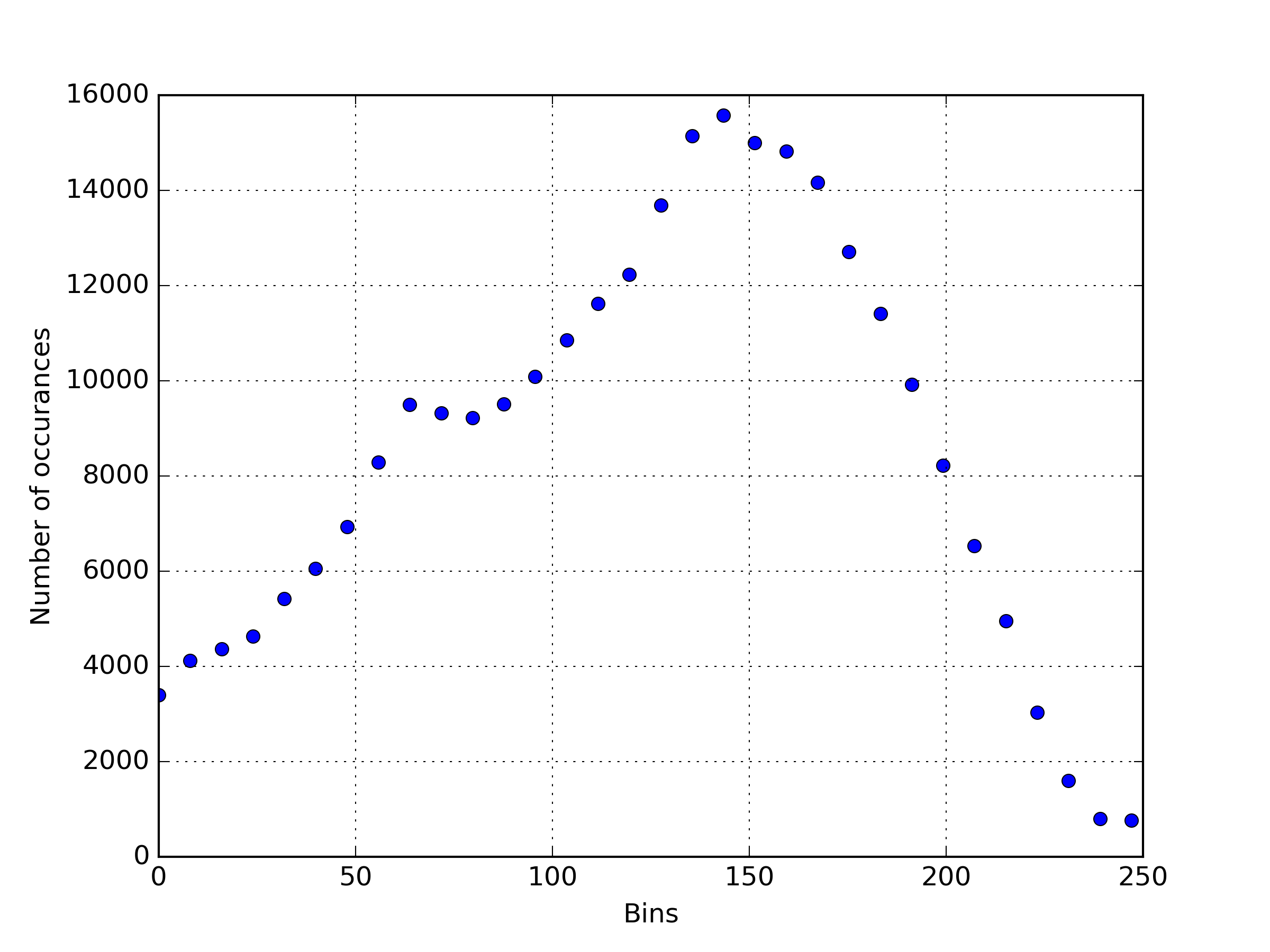 As you can see, the histogram looks nothing like the image of the dog. The theory in this work is that I have enough data to find a pattern in the histograms of Tinder profiles that I have Liked, to successfully predict future Likes.
Now an interesting problem is how to deal with the multiple photos of each Tinder profile. One simple solution would be to just take the first picture from each user. I chose not do this, because with my custom application I saw every profile image before decided to either Like or Dislike. I thought of two different methods to combine multiple images for a single user. The first would take the average of each particular bin’s value, thus creating a resulting average histogram. The second method rather summed the values of each bin to create a single summed histogram. Both the average and sum methods were used with a support vector machine to create an image classification model, however no difference was observed between the two methods.
Support vector machine
The sci-kit learn Python library [2] was used to create the support vector machine. Separate classification models were created for the values of the histogram bins from the average and sum method, to understand if one method of dealing with multiple images was superior to the other. The variables used for the classification model are the values of the histogram bins, while the output is either a Like or Dislike.
Sci-kit learn’s support vector classification supports linear, polynomial, radial basis function, sigmoid, and custom kernel functions. For this initial investigation, support vector machines were created for the built-in kernel functions. It may be interesting to apply a custom kernel function to this image classification problem in the future.
If we just fit the default support vector machine (which uses the radial basis functions) to the dataset as-is, we find that the classification model is capable of predicting over 99.9% of the Tinder profiles I’ve browsed. This was exciting news, however my model is extremely over fitting the data!
There are two options I explored simultaneously to deal with over fitting. Scaling the variable values and fine tuning the C penalty parameter in the support vector machine. The lower the C value, the smoother the classification surface. The higher the C value, the more the model is likely to attempt to classify each individual point if possible. By scaling the variables and adjusting the C parameter, I was able to find a model that matched 90% of the Tinder profiles I browsed. However 10-fold cross validation demonstrated that the parameters for this model generalized very poorly, having a 10-fold mean prediction accuracy of 63.2% with a standard deviation of 0.99%.
The goal of classification problems is to create a model that generalizes the entire population well. In this case instead of the entire population, we have only a limited sample of 8,500 data points. It is an ever-so-delicate balancing act to find a model that doesn’t over fit the data while being able to generalize the entire population well.
I continued to tweak my variable scaling technique and C penalty parameter in hopes of finding a support vector classification model capable of generalizing my dataset. A differential optimization was run with a population of 20 on different kernel functions, attempting to maximize the 10-fold cross validation mean prediction accuracy. The hope was that an optimal C penalty parameter could be found.
Results
The results of the differential evolution optimizations demonstrated some important findings. The kernel function chosen didn’t seem to affect the accuracy of the support vector classification, mostly due to the fact that my resultant model was nearly a linear cut through the design space. Additionally it appears that the sum and mean histogram methods produce equivalent classification models. In Table 1. the average 10-fold cross validation prediction accuracy is shown, and it can be seen that all models are equivalent with 71.05% prediction accuracy. Table 2. shows the optimally determined C penalty parameters for each model, which in my case was a value in the hundreds.
Table 1. Average 10-fold cross validation prediction accuracy in percent.
| Kernel function | Average histogram | Sum histogram |
| Linear | 71.05 | 71.05 |
| Polynomial | 71.05 | 71.05 |
| Radial Basis | 71.05 | 71.05 |
| Sigmoid | 71.05 | 71.05 |
Table 2. Optimal determined C penalty parameter.
| Kernel function | Average histogram | Sum histogram |
| Linear | 633 | 228 |
| Polynomial | 825 | 338 |
| Radial Basis | 448 | 225 |
| Sigmoid | 1619 | 836 |
It is not recommended to use differential evolution to determine the optimal C penalty parameter. In my experience the exact value of C did not greatly affect the results of the support vector classification model. Rather focus on finding what order of magnitude works as a stable C value. If finding an optimal C value is very important to you, I recommend using a gradient optimization method (BFGS). It is suspected that much fewer function evaluations would have been performed had I used BFGS instead of differential evolution. This is because gradient optimization can find a suitable search direction for a one variable problem with only two function evaluations.
The final chosen support vector classification model was able to match 71.05% of my Likes and Dislikes of the 8,500 Tinder profiles I browsed. The model had a mean 10-fold cross validation prediction accuracy of 71.05%, with a standard deviation of 1.5%. With some very generous assumptions, my 95% confidence interval on my model’s accuracy is 71.05% ± 3%. It was assumed that the model generalizes the entire population well, since the cross validation accuracy was very similar to accuracy of the entire dataset. Though the actual accuracy of the model on the entire population will always be unknown. Implementation of the support vector machine to automatically Like and Dislike Tinder profiles based on my personal preference is simple task with the custom application.
Conclusion
A custom application was built using the pynder Python library to record 8,500 Likes and Dislikes on Tinder profiles. Using a Histogram approach inspired by the one described in [1], support vector machines were used to perform image classification on the recorded Tinder profile images. The classification model predicts whether I’ll personally Like or Dislike a profile to about 71% accuracy. I believe that such a high prediction accuracy demonstrates that the method was successful. Very little effort is required to implement the support vector classification model into the custom application, such that the model can Like profiles based on my historical preference.
This was just an initial investigation, with many avenues to explore for future work. Since the resulting support vector machine was very linear, simplifying the classification model to a very simple linear model may have great benefits. For instance, a simpler model would be quicker at training and testing.
Variable scaling is incredibly important, and the final model wouldn’t be possible without some form of scaling. It would be interesting to perform a sensitivity analysis on the histogram bin variables, to determine which bins are the most important. Additionally it will be interesting to determine how many histogram bins is optimal for this particular image classification problem. I suspect it will be a great point o interest to investigate how many data points are required to successfully apply this method.
I’m very interested in working with this data to create an even better model. If you have any ideas on what I could have done better, please get in touch. I’ll be very happy to share this data, and to collaborate on further research!
References
[1] O. Chapelle, P. Haffner and V. N. Vapnik, Support vector machines for histogram-based image classification, in IEEE Transactions on Neural Networks, vol. 10, no. 5, pp. 1055-1064, Sep 1999. doi: 10.1109/72.788646
[2] F. Pedregosa, G. Varoquaux, A. Gramfort , V. Michel, B. Thirion, O. Grisel, M. Blondel, P. Prettenhofer, R. Weiss, V. Dubourg, J. Vanderplas, A. Passos, D. Cournapeau, M. Brucher, M. Perrot, É. Duchesnay, Scikit-learn: Machine Learning in Python, Journal of Machine Learning Research, Volume 12, pages 2825–2830, 2011.