Gaussian Process Prediction (aka Kriging) with Different Correlation Functions

EDIT Oct 8, 2018: This method for fitting a Gaussian Process has been depreciated in scikit-learn. I may update this post at somepoint in time, but for now see the scikit-learn documentation.

I was looking for a Python Kriging package for the longest time, and somehow I overlooked scikit-learn. Honestly I didn’t understand that Kriging is a Gaussian process prediction (see the wiki).This post will demonstrate how to use scikit-learn to create a Kriging model (Gaussian process prediction) for a single independent variable.

Let’s say we have some function \( Y(X) \) defined as

and we would like to use Kriging to approximate the function \( Y(X) \) on the domain of \( 0 \leq X \leq 10 \) with only using 12 training points of \( x \). I didn’t pick 12 for any reason, so let’s assume these 12 points have been randomly selected. We can use sci-kit learn to easily fit a Kriging model with the following lines of Python code.

#   let's see how well a gaussian process can fit the data
from sklearn import gaussian_process
import numpy as np
import matplotlib.pyplot as plt

#   full X range
X = np.arange(0.0,10.0+.1,.1)
#   true function values
Y = (X*(np.sin(X)**3)) - (np.cos(X)/(X+.5))

#   let's pick 12 points for the training set
x = np.array([0.5, 0.87, 1.5, 2.8, 3.6, 4.8, 6.5, 6.8, 7.7, 8.4, 9.3, 9.7])
y = (x*(np.sin(x)**3)) - (np.cos(x)/(x+.5))

#   reshape numpy arrays for scikit-learn input
X = X.reshape(-1,1)
Y = Y.reshape(-1,1)
x = x.reshape(-1,1)
y = y.reshape(-1,1)

#   initiate the Gaussian process
gp = gaussian_process.GaussianProcess()
#   fit to our training points
gp.fit(x,y)
yPred, predMSE = gp.predict(X, eval_MSE=True)

#   plot X and Y
plt.figure()
plt.plot(X,Y, '-k', label=r'$Y = X \sin (X)^3 + \frac{\cos(X)}{X+0.5}$')
plt.plot(x,y, 'ok', label='Training points')
plt.plot(X, yPred, '-r', label='GP prediction')
plt.xlabel('X')
plt.ylabel('Y')
plt.grid(True)
plt.legend(loc =2)
plt.show()

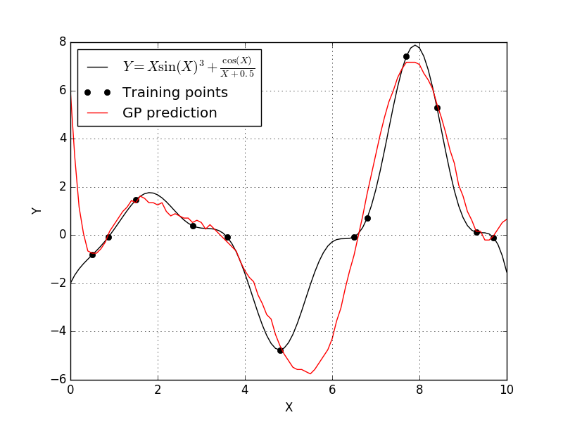
This fit is okay, but we can certainly do better. According to the scikit-learn documentation on the Gaussian process model, we notice that have a few options for the correlation function. The scikit-learn Gaussian process defaults to a squared-exponential correlation function. Let’s see what happens if we pick a different correlation function, so let’s set the correlation to absolute-exponential and see what happens.

gp = gaussian_process.GaussianProcess(corr='absolute_exponential') gp.fit(x,y)
yPred, predMSE = gp.predict(X, eval_MSE=True)

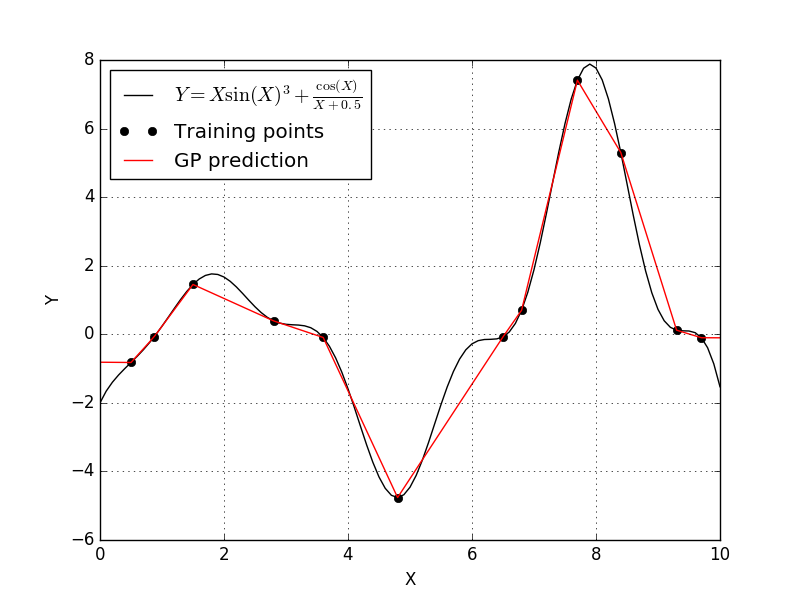
Well this isn’t a much better fit. It appears that the Absolute-exponential correlation function results in a Kriging model that linearly interpolated between our training points. So let’s try the generalized-exponential correlation function and see what happens.

gp = gaussian_process.GaussianProcess(corr='generalized_exponential')
gp.fit(x,y)
yPred, predMSE = gp.predict(X, eval_MSE=True)

Results in an error!

Exception: Length of theta must be 2 or 2

OOPS! It appears that in order to use the generalized-exponential correlation function, we needed to supply the Gaussian process with theta values. Let’s try that again.

gp = gaussian_process.GaussianProcess(corr='generalized_exponential', theta0=[1e-2,1e-2],
thetaL=[1e-3,1e-3],
thetaU=[1e-1,1e-1])
gp.fit(x,y)
yPred, predMSE = gp.predict(X, eval_MSE=True)

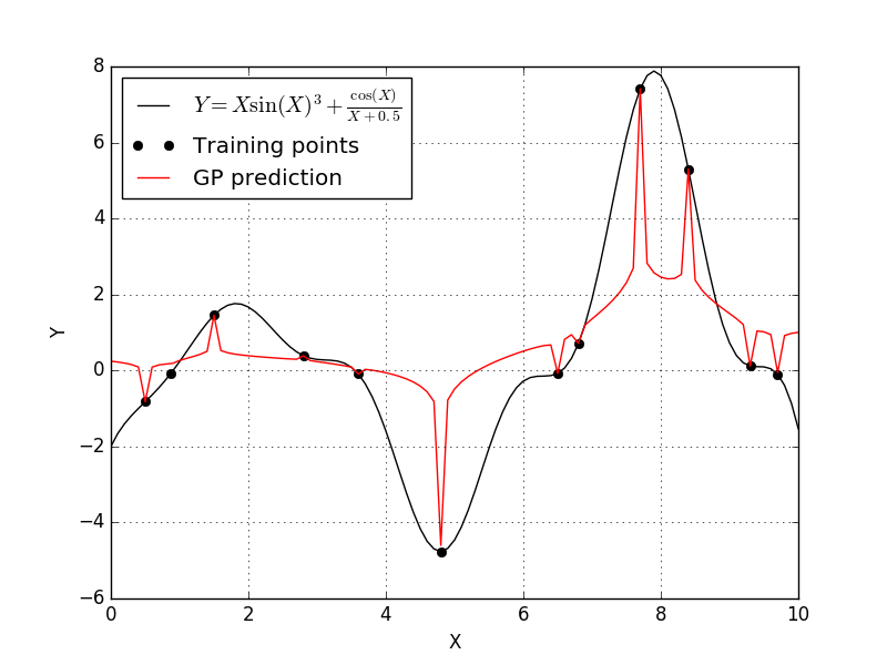
This didn’t create a great fit either. It appears that with the generalized-exponential correlation function pulled the trend down to each individual training point. Let’s now try the cubic correlation function to see what happens.

gp = gaussian_process.GaussianProcess(corr='cubic')
gp.fit(x,y)
yPred, predMSE = gp.predict(X, eval_MSE=True)

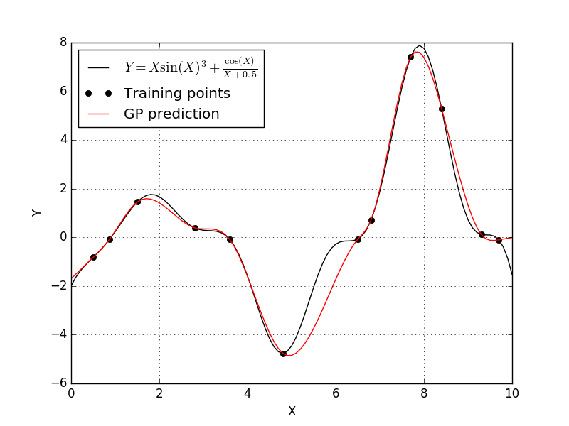
Well it looks like the cubic correlation function produces our best fit yet. The only correlation function left to try is the linear correlation function.

gp = gaussian_process.GaussianProcess(corr='linear')
gp.fit(x,y)
yPred, predMSE = gp.predict(X, eval_MSE=True)

Well the linear correlation function produced a model very similar to the absolute-exponential correlation function.

Clearly the best Kriging model used the cubic correlation function. This won’t be the case for every problem, and if you aren’t sure which correlation model to use, you could always attempt some form model selection study.