Lack of Fit Test for Linear Regression

Myers et al. [1] provides a derivation for a simple lack of fit test in section 2.7. The derivation looks at whether or not a linear model of form

adequately describes the data. Unfortunately the example provided has a mistake (while the figure matches the data, the coefficients and error values do not), so this post aims to provide corrected error values for the sample data. In addition, all of the source code to work through the problem in Python is provided here.

In order to apply the lack of fit test, we’ll need a data set that has true replicates as described in [1]. The following figure contains the data set we’ll be working with, along with the linear model fit to the data.

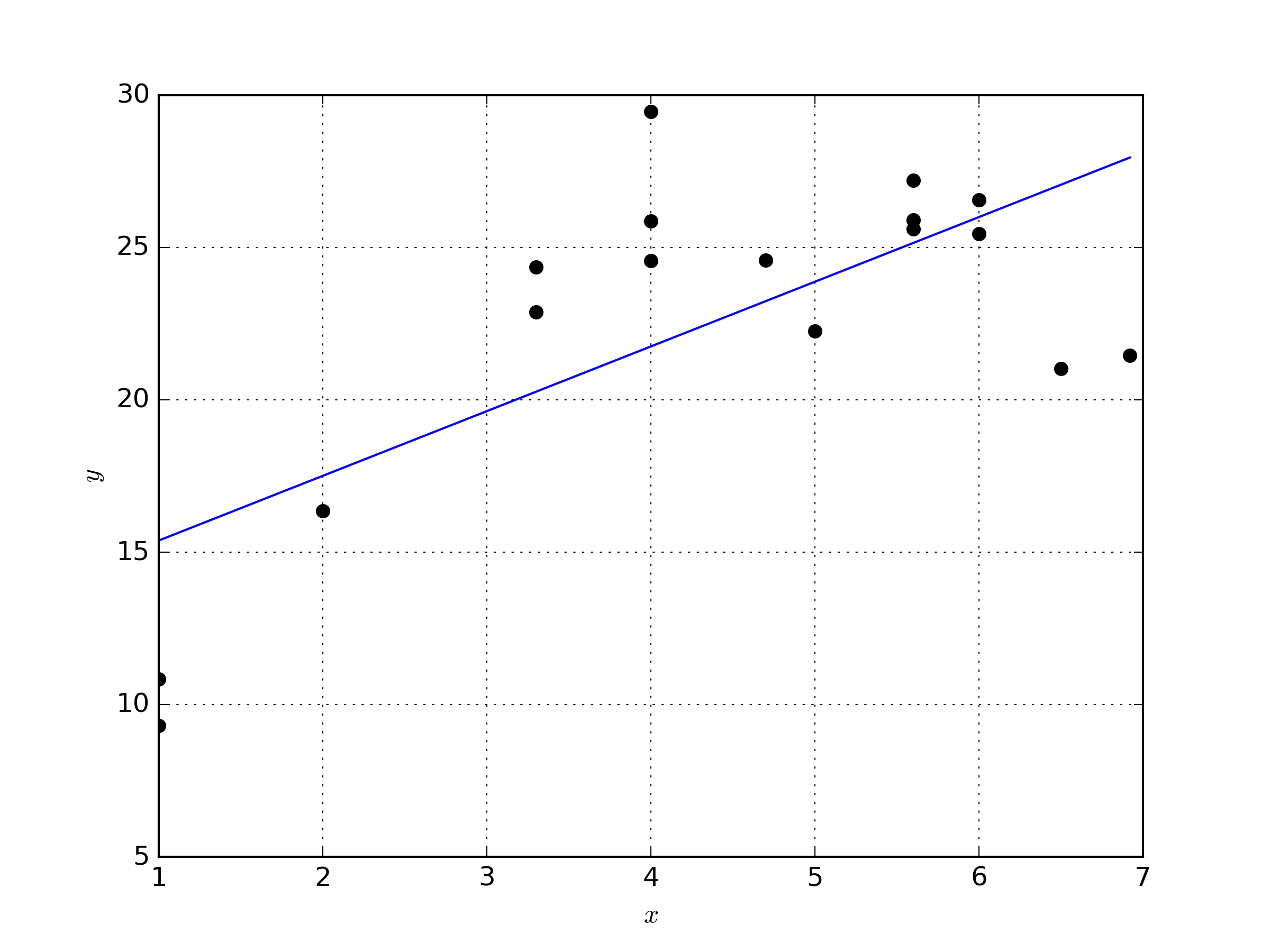
The coefficients of the linear model that were determined with a least squares fit are \( \beta_0 =13.25847151, \beta_1 = 2.12367129 \). The Python code to generate the data, create the figure, and perform the least squares fit is available below.

import numpy as np
import matplotlib.pyplot as plt
#   Create the data set
x = np.array([1.0, 1.0, 2.0, 3.3, 3.3, 4.0, 4.0, 4.0, 4.7, 5.0, 5.6,
    5.6, 5.6, 6.0, 6.0, 6.5, 6.92])
y = np.array([10.84, 9.30, 16.35, 22.88, 24.35, 24.56, 25.86, 29.46,
    24.59, 22.25, 25.90, 27.20, 25.61, 25.45, 26.56, 21.03, 21.46])

#   fit a linear model
A = np.ones([len(x), 2])
A[:,1] = x
beta, SSe, rank, s = np.linalg.lstsq(A,y)
xl = np.linspace(min(x),max(x),num=100)
Al = np.ones([len(xl), 2])
Al[:,1] = xl
yl = np.dot(Al,beta)
yhat = np.dot(A,beta)
#   plot
plt.figure()
plt.plot(x,y,'ok')
plt.plot(xl,yl,'-b')
plt.grid(True)
plt.xlabel('$x$')
plt.ylabel('$y$')
plt.show()
plt.savefig('dataAndFit.png', ftype='png', dpi=300)

As it happens, the data has \( n_i \) observations for each unique \( x_i\) level. For instance when \( x = 1.0 \), there are 2 observations of \(x\). However \( x= 2.0 \) only has 1 observation. The data has \( m \) number of levels. The residual sum of squares (the sum of squares of the residuals, in Python variable SSe returned from the linear regression) is then broken into two separate components such that

where \( SS_{PE} \) represents the sum of squares from pure error and \( SS_{LOF} \) represents the sum of squares from the lack of fit. The sum of squares from pure error is defined as

where \( y_{ij} \) is the j observation from the data at the \( x_i \) level where \( j = 1, \cdots, n_i \). Source code to calculate the sum of the squares due to pure error is provided below.

#   compute the sum of squares of pure error
level = np.array([1.0, 2.0, 3.3, 4.0, 4.7, 5.0, 5.6, 6.0, 6.5, 6.92])
levelIndex = [y[0:2], y[2], y[3:5], y[5:8], y[8], y[9],
    y[10:13], y[13:15], y[15], y[16]]
ybarLevels = []
for i in levelIndex:
    ybarLevels.append(np.mean(i))
SSpe = 0
for i, r in enumerate(levelIndex):
    SSpe += np.sum((r-ybarLevels[i])**2)

The sum of squares from lack of fit is defined as

where \( \bar{y}\) is the y mean of the i level and \( \hat{y}\) is the predicted y response at \( x_i \). The source code to calculate the sum of squares for the lack of fit is provided below.

#   compute the sum of squares lack of fit
nl = len(level)
SSlof = 0
Alevel = np.ones([nl,2])
Alevel[:,1] = level
yhatLevel = np.dot(Alevel,beta)
for i, j in enumerate(ybarLevels):
    ni = np.size(levelIndex[i])
    SSlof+= ni*((j-yhatLevel[i])**2)

We thus far have for this example that \(SS_{E} = 255.22, SS_{PE} = 17.20, SS_{LOF} = 238.02 \). It can be noted that the equation \( SS_E = SS_{PE} + SS_{LOF} \) holds true.

The test statistic \( F_0 \) to test for lack of fit is defined as

for \( p \) number of parameters. The code to calculate the test statistic is provided below.

#   Statistical test for lack of fit
m = len(ybarLevels)
n = len(x)
p = len(beta)
F0 = (SSlof / (m-p)) / (SSpe / (n-m))

We find that \( F_0 = 12.106 \) which follows the F-distribution of \( F(\alpha : m-p, n-m) \). It can be concluded that regression function is not linear because \( F_0 = 12.106 > F(\alpha : m-p, n-m) \). Alternatively the P-value for the hypothesis of \( P(F_0 \leq F(F_0: m-p, n-m) \) is 0.0018. Since the P-value is so small, the hypothesis is rejected. The P-value can be calculated with the following code:

#   test for lack of fit
from scipy.stats import f
pValue = 1.0 - f.cdf(F0,m-p,n-m)

In conclusion the linear model of \( \hat{y} = \beta_0 + \beta_1 x \) is inadequate of representing the data because most of the error results from the lack of fit, rather than pure error in the data. A better model can be constructed (potentially a higher order polynomial) to reduce the error from lack of fit.

[1] R. H. Myers, D. C. Montgomery, C. M. Anderson-Cook, Response Sur- face Methodology: Process and Product Optimization Using Designed Experiments, Wiley Series in Probability and Statistics, Wiley, ISBN 9781118916032, 2016.