Better error bars with tolerance intervals

There is a general belief that plots with error bars are superior to plots without error bars. Sometimes you’ll see people plotting error bars at +- 1.96 standard deviations, however this isn’t as statistically robust as using a tolerance interval. This post will compare error bars from the sample standard deviation to error bars from a tolerance interval. The examples use only 10 replicate data points, reflective of many cases where limited replicate data is available.

Consider 10 samples from the Normal Distribution

So let’s take a look at the following 10 samples from the standard Normal distribution.

import numpy as np
np.random.seed(111)
x = np.random.normal(size=10)
print('Sample mean: ', x.mean())
print('Sample standard deviation: ', x.std(ddof=1))

With only 10 samples, you’ll see we have a fairly poor estimation of the true mean and standard deviation, which should be zero and one respectively. If we assume that the sample mean and standard deviation are correct, and the distribution is Normal, then the mean plus-or-minus 1.96 standard deviations would bound the central 95% region of our distribution. This is related to error bars, because it implies that a new sample would have a 95% chance of landing withing the bounds.

Now since we know the sample mean and standard deviation are not correct, we can construct a tolerance interval to account for the errors in our limited random sample. We’ll use the Python toleranceinterval package to do so. The following code will find the lower and upper bound on a tolerance interval based on the previous random sample, to obtain the central 95% region to 95% confidence for a normal distribution. The confidence aspect is important, as it implies the bounds will be conservative estimates for 95% of the possible Normal distributions the random sample could have come from.

import toleranceinterval as ti
bounds = ti.twoside.normal(x, 0.95, 0.95)
print('Lower bound: ', bounds[:, 0])
print('Upper bound: ', bounds[:, 1])

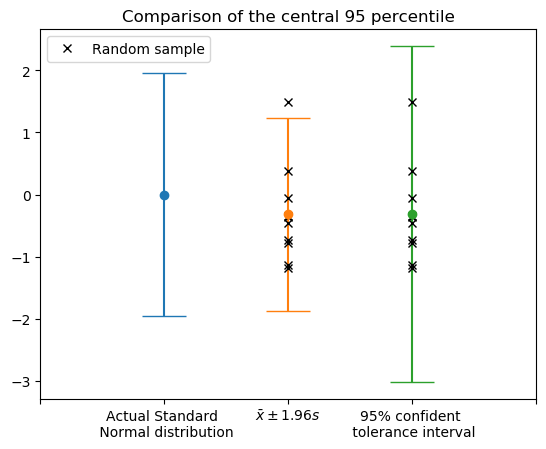
So how do the bounds differ visually? The following plot illustrates the differences between the methods. To the left we see the central 95% region of the true Normal distribution, from which the random samples were generated from. In the center, we see the sample mean plus-or-minus 1.96 times the sample standard deviation. The x points denote the locations of the 10 random samples. The bounds using the sample mean plus-or-minus 1.96 sample standard deviations results in error bounds that are less than the 95% region from the true distribution. The right most plot shows the error bounds from a two-sided tolerance interval, which are a conservative estimation of the 95% region from the true distribution.

The following code generates the above plot. One way to go from the toleranceinterval bounds to matplotlib errorbar is to set the error to be the absolute deviations from the mean, which is done with np.abs(x.mean()-bounds.T).

import matplotlib.pyplot as plt

plt.figure()
plt.title('Comparison of the central 95 percentile')
plt.errorbar(1, 0, yerr=[1.96], fmt='o', capsize=16.0)

plt.errorbar(2, x.mean(), yerr=[1.96*x.std(ddof=1)], fmt='o',
             capsize=16.0)
plt.plot(2*np.ones_like(x), x, 'xk', label='Random sample')

plt.errorbar(3, x.mean(), yerr=np.abs(x.mean()-bounds.T),
             fmt='o', capsize=16.0)
plt.plot(3*np.ones_like(x), x, 'xk')

plt.xticks(np.arange(5), ('',
                          'Actual Standard \n Normal distribution',
                          r'$\bar{x} \pm 1.96  s $',
                          '95% confident \n tolerance interval',
                          ''))
plt.legend()
plt.show()

Consider a computational benchmark with 10 replicate runs

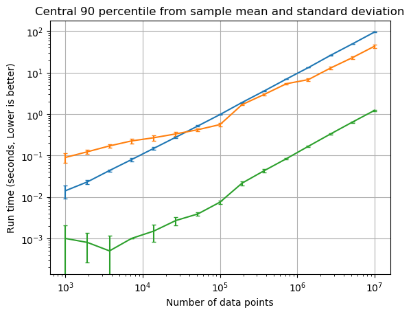
Consider the following benchmark I performed in this post, where I compute the runtime at each configuration 10 replicate times.

This first figure shows the benchmark if error bars were computed using the sample mean plus-or-minus 1.282 times the sample standard deviation. The 1.282 times the standard deviation represents the central 90% of a Normal distribution.

This follow up figure shows the benchmark if error bars were computed using a two-sided Normal tolerance interval. The tolerance interval shows the bounds for the central 90% to 95% confidence. The difference is fairly drastic where the variance in replicates was large, as the tolerance interval has much larger error bounds. Also the sample mean plus-or-minus 1.282 times the sample standard deviation was likely underestimating the central 90th percentile.

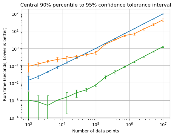
In this case whether we used the two-sided tolerance interval, or used a rudimentary multiplier on the sample mean and standard deviation, the conclusion on which method was faster would be the same. The difference is with the tolerance interval method we have some basis to state the the observed speed difference was statistically significant.

Conclusion

If you want to have some statistical assurance in error bounds of a random sample, you may want to consider using a tolerance interval. This post showed how to use the toleranceinterval package to generate these two-sided error bounds for a normal distribution. I’ll save what to do if you don’t know the true distribution for another time!