Ellipsoid Non-linear Regression Fitting
December 4, 2021
In one of my previous posts, I demonstrated how to fit an ellipsoid using least squares. Unfortunately, this method won’t work for many practical problems because the data will not be centered around the origin. For these cases, we will need to formulate a more expensive non-linear regression problem that uses optimization to find the ellipsoid parameters. We will use jax.numpy as an automatic differentiation code to easily compute derivatives for our custom non-linear regression.
Mathematical preliminaries
So an arbitrary ellipsoid in 3D space can be defined as
where our ellipsoid parameters are \( x_0 \), \( y_0 \), \( z_0 \), \( a \), \( b \), and \( c \). We can then setup an optimization formulation to find the best six parameters to some arbitrary collection of data in 3D space. There will be some error for any given set of ellipsoid parameters on our data. Optimization will then be used to find the six parameters that minimizes this error.
Let \( \hat{f} \) represent some arbitrary candidate ellipsoid as
We can define some error function which represents how far \( \hat{f} \) deviates from 1 for our observed \( x_i \), \( y_i \), and \( z_i \) data. We are going to use the mean squared error which is a \( L^2 \) norm that is differentiable everywhere. The mean squared error for our ellipsoid fitting will be defined as
for \( n \) data points. Now we can define an optimization problem to find \( [\gamma_0, \gamma_1, \gamma_2, \gamma_3, \gamma_4, \gamma_5] \) that minimizes \( e \).
This isn’t a perfect formulation to fit ellipsoids because the formulation is not convex if there are no bounds on \( [\gamma_0, \gamma_1, \gamma_2, \gamma_3, \gamma_4, \gamma_5] \). In other words, you can imagine that for any data set their exists some enormous ellipsoid (think infinite radius) that just barely graces your data. These enormous ellipsoids will have a mean squared error of 0, which is the lowest possible error.
The key to get this formulation to work is to guess \( [\gamma_0, \gamma_1, \gamma_2, \gamma_3, \gamma_4, \gamma_5] \) reasonably. While it may not be easy to guess \( a \), \( b \), and \( c \), it is very easy to guess the center of the ellipse. In my case I just take the mean of the observed data to guess the centroid of the ellipse.
Example Ellipsoid Data
Consider the following example ellipsoid data with some amount of noise,
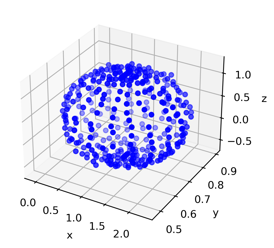
which is generated from the following Python code
import numpy as np
import matplotlib.pyplot as plt
from mpl_toolkits.mplot3d import Axes3D

n_one = 20
np.random.seed(123)
noise = np.random.normal(size=(n_one*n_one), loc=0, scale=1e-2)

u = np.linspace(0., np.pi*2., n_one)
v = np.linspace(0., np.pi, n_one)
u, v = np.meshgrid(u,v)
a = 1.2
b = 0.2
c = 0.9
x = a*np.cos(u)*np.sin(v)
y = b*np.sin(u)*np.sin(v)
z = c*np.cos(v)

x = x.flatten() + noise
y = y.flatten() + noise
z = z.flatten() + noise

x0 = 1.1
y0 = 0.7
z0 = 0.3

x += x0
y += y0
z += z0
Automatic Differentiation with JAX
We will need derivatives of \( e \) in order to find the optimum ellipsoid parameters. Writing the correct derivative used to be the most difficult part of many non-linear regression applications. However with the abundance of automatic differentiation (AD) codes, writing the derivatives of our ellipsoid fitting routine is automatic! We will just need to write out code that computes \( e \) as a function of \( [\gamma_0, \gamma_1, \gamma_2, \gamma_3, \gamma_4, \gamma_5] \), and then let the AD do the rest.
Let’s load in JAX and come up with a guess for gamma. We use the mean observed values to guess the center of the ellipsoid, and simply use random values to guess \( a \), \( b \), and \( c \).
import jax.numpy as jnp
from jax import grad
from jax import random
from jax.config import config
config.update('jax_enable_x64', True)
key = random.PRNGKey(0)

gamma_guess = np.random.random(6)
gamma_guess[0] = x.mean()
gamma_guess[1] = y.mean()
gamma_guess[2] = z.mean()
gamma_guess = jnp.array(gamma_guess)

print(gamma_guess)
Which prints [1.13565174 0.69944713 0.29944713 0.91947247 0.41550355 0.74461546].
We can then define our mean squared error (\( e \)) objective function as the following.
def predict(gamma):
    # compute f hat
    x0 = gamma[0]
    y0 = gamma[1]
    z0 = gamma[2]
    a2 = gamma[3]**2
    b2 = gamma[4]**2
    c2 = gamma[5]**2
    zeta0 = (x - x0)**2 / a2
    zeta1 = (y - y0)**2 / b2
    zeta2 = (z - z0)**2 / c2
    return zeta0 + zeta1 + zeta2


def loss(g):
    # compute mean squared error
    pred = predict(g)
    target = jnp.ones_like(pred)
    mse = jnp.square(pred-target).mean()
    return mse


print(loss(gamma_guess))
Which gives us an initial mean squared error of 0.18875287. We will need to compute the derivatives of the mean squared error with respect to each gamma component. This is
and can simply be calculated with JAX in one line of code!
print(grad(loss)(gamma_guess))
which gives us [0.07587903, -0.00453702, -0.00563972, -0.72330367, 0.08752203, -1.49206736].
Optimization
We will use BFGS to find our ellipsoid parameters that minimize \( e \). This is done in Python using the following code.
from scipy.optimize import fmin_bfgs

res = fmin_bfgs(
    loss,
    gamma_guess,
    fprime=grad(loss),
    norm=2.0,
    args=(),
    gtol=1e-17,
    maxiter=None,
    full_output=1,
    disp=1,
    retall=0,
    callback=None
)
print(res)
Which gives us the following result
| Parameter | Ellipsoid Fit | Actual solution |
|---|---|---|
| \( x_0 \) | 1.10197386 | 1.1 |
| \( y_0 \) | 0.69957001 | 0.7 |
| \( z_0 \) | 0.30146653 | 0.3 |
| \( a \) | 1.19767917 | 1.2 |
| \( b \) | 0.20274865 | 0.2 |
| \( c \) | 0.90162033 | 0.9 |
You’ll notice that the result is very close to our actual ellipse values! The following figure shows the fitted ellipsoid and the data.
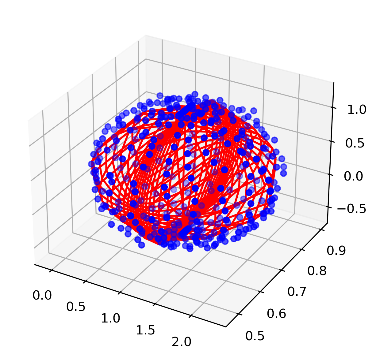
If you run into problems where \( e \) is going to zero, you are probably running into the convexity issue I mentioned earlier. In these cases I’d suggest trying to come up with bounds around the six ellipsoid parameters, and then using a bounded optimization algorithm like L-BFGS-B.
The full Python code of this work can be found here.