Examples

All of these examples will use the following data and imports.

import numpy as np
import matplotlib.pyplot as plt
import pwlf

# your data
y = np.array([0.00000000e+00, 9.69801700e-03, 2.94350340e-02,
              4.39052750e-02, 5.45343950e-02, 6.74104940e-02,
              8.34831790e-02, 1.02580042e-01, 1.22767939e-01,
              1.42172312e-01, 0.00000000e+00, 8.58600000e-06,
              8.31543400e-03, 2.34184100e-02, 3.39709150e-02,
              4.03581990e-02, 4.53545600e-02, 5.02345260e-02,
              5.55253360e-02, 6.14750770e-02, 6.82125120e-02,
              7.55892510e-02, 8.38356810e-02, 9.26413070e-02,
              1.02039790e-01, 1.11688258e-01, 1.21390666e-01,
              1.31196948e-01, 0.00000000e+00, 1.56706510e-02,
              3.54628780e-02, 4.63739040e-02, 5.61442590e-02,
              6.78542550e-02, 8.16388310e-02, 9.77756110e-02,
              1.16531753e-01, 1.37038283e-01, 0.00000000e+00,
              1.16951050e-02, 3.12089850e-02, 4.41776550e-02,
              5.42877590e-02, 6.63321350e-02, 8.07655920e-02,
              9.70363280e-02, 1.15706975e-01, 1.36687642e-01,
              0.00000000e+00, 1.50144640e-02, 3.44519970e-02,
              4.55907760e-02, 5.59556700e-02, 6.88450940e-02,
              8.41374060e-02, 1.01254006e-01, 1.20605073e-01,
              1.41881288e-01, 1.62618058e-01])
x = np.array([0.00000000e+00, 8.82678000e-03, 3.25615100e-02,
              5.66106800e-02, 7.95549800e-02, 1.00936330e-01,
              1.20351520e-01, 1.37442010e-01, 1.51858250e-01,
              1.64433570e-01, 0.00000000e+00, -2.12600000e-05,
              7.03872000e-03, 1.85494500e-02, 3.00926700e-02,
              4.17617000e-02, 5.37279600e-02, 6.54941000e-02,
              7.68092100e-02, 8.76596300e-02, 9.80525800e-02,
              1.07961810e-01, 1.17305210e-01, 1.26063930e-01,
              1.34180360e-01, 1.41725010e-01, 1.48629710e-01,
              1.55374770e-01, 0.00000000e+00, 1.65610200e-02,
              3.91016100e-02, 6.18679400e-02, 8.30997400e-02,
              1.02132890e-01, 1.19011260e-01, 1.34620080e-01,
              1.49429370e-01, 1.63539960e-01, -0.00000000e+00,
              1.01980300e-02, 3.28642800e-02, 5.59461900e-02,
              7.81388400e-02, 9.84458400e-02, 1.16270210e-01,
              1.31279040e-01, 1.45437090e-01, 1.59627540e-01,
              0.00000000e+00, 1.63404300e-02, 4.00086000e-02,
              6.34390200e-02, 8.51085900e-02, 1.04787860e-01,
              1.22120350e-01, 1.36931660e-01, 1.50958760e-01,
              1.65299640e-01, 1.79942720e-01])

1. fit with known breakpoint locations

2. fit for specified number of line segments

3. fitfast for specified number of line segments

4. force a fit through data points

5. use custom optimization routine

6. pass differential evolution keywords

7. find the best number of line segments

8. model persistence

9. bad fits when you have more unknowns than data

10. fit with a breakpoint guess

11. get the linear regression matrix

12. use of TensorFlow

13. fit constants or polynomials

14. specify breakpoint bounds

15. non-linear standard errors and p-values

16. obtain the equations of fitted pwlf

17. weighted least squares fit

18. reproducible results

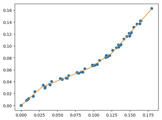
fit with known breakpoint locations

You can perform a least squares fit if you know the breakpoint locations.

# your desired line segment end locations
x0 = np.array([min(x), 0.039, 0.10, max(x)])

# initialize piecewise linear fit with your x and y data
my_pwlf = pwlf.PiecewiseLinFit(x, y)

# fit the data with the specified break points
# (ie the x locations of where the line segments
# will terminate)
my_pwlf.fit_with_breaks(x0)

# predict for the determined points
xHat = np.linspace(min(x), max(x), num=10000)
yHat = my_pwlf.predict(xHat)

# plot the results
plt.figure()
plt.plot(x, y, 'o')
plt.plot(xHat, yHat, '-')
plt.show()

fit with known breakpoint locations

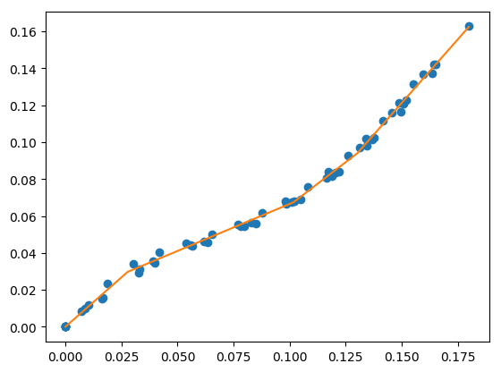
fit for specified number of line segments

Use a global optimization to find the breakpoint locations that minimize the sum of squares error. This uses Differential Evolution from scipy.

# initialize piecewise linear fit with your x and y data
my_pwlf = pwlf.PiecewiseLinFit(x, y)

# fit the data for four line segments
res = my_pwlf.fit(4)

# predict for the determined points
xHat = np.linspace(min(x), max(x), num=10000)
yHat = my_pwlf.predict(xHat)

# plot the results
plt.figure()
plt.plot(x, y, 'o')
plt.plot(xHat, yHat, '-')
plt.show()

fit for specified number of line segments

fitfast for specified number of line segments

This performs a fit for a specified number of line segments with a multi-start gradient based optimization. This should be faster than Differential Evolution for a small number of starting points.

# initialize piecewise linear fit with your x and y data
my_pwlf = pwlf.PiecewiseLinFit(x, y)

# fit the data for four line segments
# this performs 3 multi-start optimizations
res = my_pwlf.fitfast(4, pop=3)

# predict for the determined points
xHat = np.linspace(min(x), max(x), num=10000)
yHat = my_pwlf.predict(xHat)

# plot the results
plt.figure()
plt.plot(x, y, 'o')
plt.plot(xHat, yHat, '-')
plt.show()

fitfast for specified number of line segments

force a fit through data points

Sometimes it’s necessary to force the piecewise continuous model through a particular data point, or a set of data points. The following example finds the best 4 line segments that go through two data points.

# initialize piecewise linear fit with your x and y data
myPWLF = pwlf.PiecewiseLinFit(x, y)

# fit the function with four line segments
# force the function to go through the data points
# (0.0, 0.0) and (0.19, 0.16)
# where the data points are of the form (x, y)
x_c = [0.0, 0.19]
y_c = [0.0, 0.2]
res = myPWLF.fit(4, x_c, y_c)

# predict for the determined points
xHat = np.linspace(min(x), 0.19, num=10000)
yHat = myPWLF.predict(xHat)

# plot the results
plt.figure()
plt.plot(x, y, 'o')
plt.plot(xHat, yHat, '-')
plt.show()

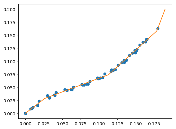
force a fit through data points

use custom optimization routine

You can use your favorite optimization routine to find the breakpoint locations. The following example uses scipy’s minimize function.

from scipy.optimize import minimize
# initialize piecewise linear fit with your x and y data
my_pwlf = pwlf.PiecewiseLinFit(x, y)

# initialize custom optimization
number_of_line_segments = 3
my_pwlf.use_custom_opt(number_of_line_segments)

# i have number_of_line_segments - 1 number of variables
# let's guess the correct location of the two unknown variables
# (the program defaults to have end segments at x0= min(x)
# and xn=max(x)
xGuess = np.zeros(number_of_line_segments - 1)
xGuess[0] = 0.02
xGuess[1] = 0.10

res = minimize(my_pwlf.fit_with_breaks_opt, xGuess)

# set up the break point locations
x0 = np.zeros(number_of_line_segments + 1)
x0[0] = np.min(x)
x0[-1] = np.max(x)
x0[1:-1] = res.x

# calculate the parameters based on the optimal break point locations
my_pwlf.fit_with_breaks(x0)

# predict for the determined points
xHat = np.linspace(min(x), max(x), num=10000)
yHat = my_pwlf.predict(xHat)

plt.figure()
plt.plot(x, y, 'o')
plt.plot(xHat, yHat, '-')
plt.show()

pass differential evolution keywords

You can pass keyword arguments from the fit function into scipy’s Differential Evolution.

# initialize piecewise linear fit with your x and y data
my_pwlf = pwlf.PiecewiseLinFit(x, y)

# fit the data for four line segments
# this sets DE to have an absolute tolerance of 0.1
res = my_pwlf.fit(4, atol=0.1)

# predict for the determined points
xHat = np.linspace(min(x), max(x), num=10000)
yHat = my_pwlf.predict(xHat)

# plot the results
plt.figure()
plt.plot(x, y, 'o')
plt.plot(xHat, yHat, '-')
plt.show()

find the best number of line segments

This example uses EGO (bayesian optimization) and a penalty function to find the best number of line segments. This will require careful use of the penalty parameter l. Use this template to automatically find the best number of line segments.

from GPyOpt.methods import BayesianOptimization
# initialize piecewise linear fit with your x and y data
my_pwlf = pwlf.PiecewiseLinFit(x, y)

# define your objective function


def my_obj(x):
    # define some penalty parameter l
    # you'll have to arbitrarily pick this
    # it depends upon the noise in your data,
    # and the value of your sum of square of residuals
    l = y.mean()*0.001
    f = np.zeros(x.shape[0])
    for i, j in enumerate(x):
        my_pwlf.fit(j[0])
        f[i] = my_pwlf.ssr + (l*j[0])
    return f


# define the lower and upper bound for the number of line segments
bounds = [{'name': 'var_1', 'type': 'discrete',
           'domain': np.arange(2, 40)}]

np.random.seed(12121)

myBopt = BayesianOptimization(my_obj, domain=bounds, model_type='GP',
                              initial_design_numdata=10,
                              initial_design_type='latin',
                              exact_feval=True, verbosity=True,
                              verbosity_model=False)
max_iter = 30

# perform the bayesian optimization to find the optimum number
# of line segments
myBopt.run_optimization(max_iter=max_iter, verbosity=True)

print('\n \n Opt found \n')
print('Optimum number of line segments:', myBopt.x_opt)
print('Function value:', myBopt.fx_opt)
myBopt.plot_acquisition()
myBopt.plot_convergence()

# perform the fit for the optimum
my_pwlf.fit(myBopt.x_opt)
# predict for the determined points
xHat = np.linspace(min(x), max(x), num=10000)
yHat = my_pwlf.predict(xHat)

# plot the results
plt.figure()
plt.plot(x, y, 'o')
plt.plot(xHat, yHat, '-')
plt.show()

model persistence

You can save fitted models with pickle. Alternatively see joblib.

# if you use Python 2.x you should import cPickle
# import cPickle as pickle
# if you use Python 3.x you can just use pickle
import pickle

# your desired line segment end locations
x0 = np.array([min(x), 0.039, 0.10, max(x)])

# initialize piecewise linear fit with your x and y data
my_pwlf = pwlf.PiecewiseLinFit(x, y)

# fit the data with the specified break points
my_pwlf.fit_with_breaks(x0)

# save the fitted model
with open('my_fit.pkl', 'wb') as f:
    pickle.dump(my_pwlf, f, pickle.HIGHEST_PROTOCOL)

# load the fitted model
with open('my_fit.pkl', 'rb') as f:
    my_pwlf = pickle.load(f)

bad fits when you have more unknowns than data

You can get very bad fits with pwlf when you have more unknowns than data points. The following example will fit 99 line segments to the 59 data points. While this will result in an error of zero, the model will have very weird predictions within the data. You should not fit more unknowns than you have data with pwlf!

break_locations = np.linspace(min(x), max(x), num=100)
# initialize piecewise linear fit with your x and y data
my_pwlf = pwlf.PiecewiseLinFit(x, y)
my_pwlf.fit_with_breaks(break_locations)

# predict for the determined points
xHat = np.linspace(min(x), max(x), num=10000)
yHat = my_pwlf.predict(xHat)

# plot the results
plt.figure()
plt.plot(x, y, 'o')
plt.plot(xHat, yHat, '-')
plt.show()

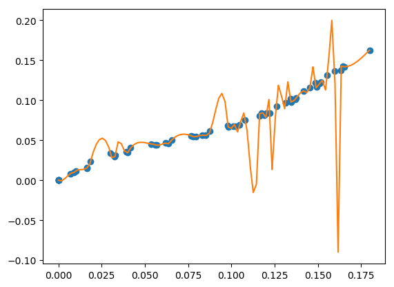
bad fits when you have more unknowns than data

fit with a breakpoint guess

In this example we see two distinct linear regions, and we believe a breakpoint occurs at 6.0. We’ll use the fit_guess() function to find the best breakpoint location starting with this guess. These fits should be much faster than the fit or fitfast function when you have a reasonable idea where the breakpoints occur.

import numpy as np
import pwlf
x = np.array([4., 5., 6., 7., 8.])
y = np.array([11., 13., 16., 28.92, 42.81])
my_pwlf = pwlf.PiecewiseLinFit(x, y)
breaks = my_pwlf.fit_guess([6.0])

Note specifying one breakpoint will result in two line segments. If we wanted three line segments, we’ll have to specify two breakpoints.

breaks = my_pwlf.fit_guess([5.5, 6.0])

get the linear regression matrix

In some cases it may be desirable to work with the linear regression matrix directly. The following example grabs the linear regression matrix A for a specific set of breakpoints. In this case we assume that the breakpoints occur at each of the data points. Please see the paper for details about the regression matrix A.

import numpy as np
import pwlf
# select random seed for reproducibility
np.random.seed(123)
# generate sin wave data
x = np.linspace(0, 10, num=100)
y = np.sin(x * np.pi / 2)
ytrue = y.copy()
# add noise to the data
y = np.random.normal(0, 0.05, 100) + ytrue

my_pwlf_en = pwlf.PiecewiseLinFit(x, y)
# copy the x data to use as break points
breaks = my_pwlf_en.x_data.copy()
# create the linear regression matrix A
A = my_pwlf_en.assemble_regression_matrix(breaks, my_pwlf_en.x_data)

We can perform fits that are more complicated than a least squares fit when we have the regression matrix. The following uses the Elastic Net regularizer to perform an interesting fit with the regression matrix.

from sklearn.linear_model import ElasticNetCV
# set up the elastic net
en_model = ElasticNetCV(cv=5,
                        l1_ratio=[.1, .5, .7, .9,
                                  .95, .99, 1],
                        fit_intercept=False,
                        max_iter=1000000, n_jobs=-1)
# fit the model using the elastic net
en_model.fit(A, my_pwlf_en.y_data)

# predict from the elastic net parameters
xhat = np.linspace(x.min(), x.max(), 1000)
yhat_en = my_pwlf_en.predict(xhat, breaks=breaks,
                             beta=en_model.coef_)

interesting elastic net fit

use of tensorflow

You need to install pwlftf which will have the PiecewiseLinFitTF class. For performance benchmarks (these benchmarks are outdated! and the regular pwlf may be faster in many applications) see this blog post.

The use of the TF class is nearly identical to the original class, however note the following exceptions. PiecewiseLinFitTF does:

• not have a lapack_driver option

• have an optional parameter dtype, so you can choose between the float64 and float32 data types

• have an optional parameter fast to switch between Cholesky decomposition (default fast=True), and orthogonal decomposition (fast=False)

import pwlftf as pwlf
# your desired line segment end locations
x0 = np.array([min(x), 0.039, 0.10, max(x)])

# initialize TF piecewise linear fit with your x and y data
my_pwlf = pwlf.PiecewiseLinFitTF(x, y, dtype='float32)

# fit the data with the specified break points
# (ie the x locations of where the line segments
# will terminate)
my_pwlf.fit_with_breaks(x0)

# predict for the determined points
xHat = np.linspace(min(x), max(x), num=10000)
yHat = my_pwlf.predict(xHat)

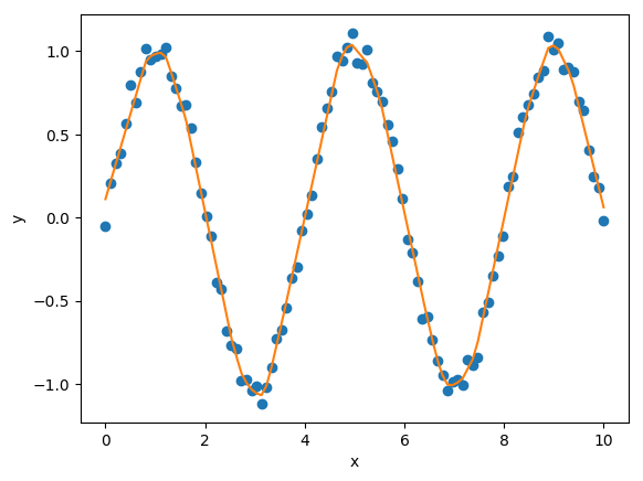
fit constants or polynomials

You can use pwlf to fit segmented constant models, or piecewise polynomials. The following example fits a segmented constant model, piecewise linear, and a piecewise quadratic model to a sine wave.

# generate sin wave data
x = np.linspace(0, 10, num=100)
y = np.sin(x * np.pi / 2)
# add noise to the data
y = np.random.normal(0, 0.05, 100) + y

# initialize piecewise linear fit with your x and y data
# pwlf lets you fit continuous model for many degree polynomials
# degree=0 constant
# degree=1 linear (default)
# degree=2 quadratic
my_pwlf_0 = pwlf.PiecewiseLinFit(x, y, degree=0)
my_pwlf_1 = pwlf.PiecewiseLinFit(x, y, degree=1)  # default
my_pwlf_2 = pwlf.PiecewiseLinFit(x, y, degree=2)

# fit the data for four line segments
res0 = my_pwlf_0.fitfast(5, pop=50)
res1 = my_pwlf_1.fitfast(5, pop=50)
res2 = my_pwlf_2.fitfast(5, pop=50)

# predict for the determined points
xHat = np.linspace(min(x), max(x), num=10000)
yHat0 = my_pwlf_0.predict(xHat)
yHat1 = my_pwlf_1.predict(xHat)
yHat2 = my_pwlf_2.predict(xHat)

# plot the results
plt.figure()
plt.plot(x, y, 'o', label='Data')
plt.plot(xHat, yHat0, '-', label='degree=0')
plt.plot(xHat, yHat1, '--', label='degree=1')
plt.plot(xHat, yHat2, ':', label='degree=2')
plt.legend()
plt.show()

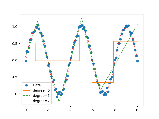
Example of multiple degree fits to a sine wave.

specify breakpoint bounds

You may want extra control over the search space for feasible breakpoints. One way to do this is to specify the bounds for each breakpoint location.

# generate sin wave data
x = np.linspace(0, 10, num=100)
y = np.sin(x * np.pi / 2)
# add noise to the data
y = np.random.normal(0, 0.05, 100) + y

# initialize piecewise linear fit with your x and y data
my_pwlf = pwlf.PiecewiseLinFit(x, y)

# define custom bounds for the interior break points
n_segments = 4
bounds = np.zeros((n_segments-1, 2))
# first breakpoint
bounds[0, 0] = 0.0  # lower bound
bounds[0, 1] = 3.5  # upper bound
# second breakpoint
bounds[1, 0] = 3.0  # lower bound
bounds[1, 1] = 7.0  # upper bound
# third breakpoint
bounds[2, 0] = 6.0  # lower bound
bounds[2, 1] = 10.0  # upper bound
res = my_pwlf.fit(n_segments, bounds=bounds)

non-linear standard errors and p-values

You can calculate non-linear standard errors using the Delta method. This will calculate the standard errors of the piecewise linear parameters (intercept + slopes) and the breakpoint locations!

First let us generate true piecewise linear data.

from __future__ import print_function
# generate a true piecewise linear data
np.random.seed(5)
n_data = 100
x = np.linspace(0, 1, num=n_data)
y = np.random.random(n_data)
my_pwlf_gen = pwlf.PiecewiseLinFit(x, y)
true_beta = np.random.normal(size=5)
true_breaks = np.array([0.0, 0.2, 0.5, 0.75, 1.0])
y = my_pwlf_gen.predict(x, beta=true_beta, breaks=true_breaks)

plt.figure()
plt.title('True piecewise linear data')
plt.plot(x, y)
plt.show()

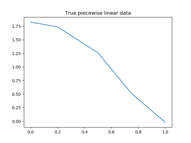
True piecewise linear data.

Now we can perform a fit, calculate the standard errors, and p-values. The non-linear method uses a first order taylor series expansion to linearize the non-linear regression problem. A positive step_size performs a forward difference, and a negative step_size would perform a backwards difference.

my_pwlf = pwlf.PiecewiseLinFit(x, y)
res = my_pwlf.fitfast(4, pop=100)

p = my_pwlf.p_values(method='non-linear', step_size=1e-4)
se = my_pwlf.se  # standard errors

The standard errors and p-values correspond to each model parameter. First the beta parameters (intercept + slopes) and then the breakpoints. We can assemble the parameters, and print a table of the result with the following code.

parameters = np.concatenate((my_pwlf.beta,
                             my_pwlf.fit_breaks[1:-1]))

header = ['Parameter type', 'Parameter value', 'Standard error', 't',
          'P > np.abs(t) (p-value)']
print(*header, sep=' | ')
values = np.zeros((parameters.size, 5), dtype=np.object_)
values[:, 1] = np.around(parameters, decimals=3)
values[:, 2] = np.around(se, decimals=3)
values[:, 3] = np.around(parameters / se, decimals=3)
values[:, 4] = np.around(p, decimals=3)

for i, row in enumerate(values):
    if i < my_pwlf.beta.size:
        row[0] = 'Beta'
        print(*row, sep=' | ')
    else:
        row[0] = 'Breakpoint'
        print(*row, sep=' | ')

Parameter type	Parameter value	Standard error	t	P > np.abs(t) (p-value)
Beta	1.821	0.0	1763191476.046	0.0
Beta	-0.427	0.0	-46404554.493	0.0
Beta	-1.165	0.0	-111181494.162	0.0
Beta	-1.397	0.0	-168954500.421	0.0
Beta	0.873	0.0	93753841.242	0.0
Breakpoint	0.2	0.0	166901856.885	0.0
Breakpoint	0.5	0.0	537785803.646	0.0
Breakpoint	0.75	0.0	482311769.159	0.0

obtain the equations of fitted pwlf

Sometimes you may want the mathematical equations that represent your fitted model. This is easy to perform if you don’t mind using sympy.

The following code will fit 5 line segments of degree=2 to a sin wave.

import numpy as np
import pwlf
# generate sin wave data
x = np.linspace(0, 10, num=100)
y = np.sin(x * np.pi / 2)
# add noise to the data
y = np.random.normal(0, 0.05, 100) + y
my_pwlf_2 = pwlf.PiecewiseLinFit(x, y, degree=2)
res2 = my_pwlf_2.fitfast(5, pop=50)

Given this fit, the following code will print the mathematical equation for each line segment.

from sympy import Symbol
from sympy.utilities import lambdify
x = Symbol('x')


def get_symbolic_eqn(pwlf_, segment_number):
    if pwlf_.degree < 1:
        raise ValueError('Degree must be at least 1')
    if segment_number < 1 or segment_number > pwlf_.n_segments:
        raise ValueError('segment_number not possible')
    # assemble degree = 1 first
    for line in range(segment_number):
        if line == 0:
            my_eqn = pwlf_.beta[0] + (pwlf_.beta[1])*(x-pwlf_.fit_breaks[0])
        else:
            my_eqn += (pwlf_.beta[line+1])*(x-pwlf_.fit_breaks[line])
    # assemble all other degrees
    if pwlf_.degree > 1:
        for k in range(2, pwlf_.degree + 1):
            for line in range(segment_number):
                beta_index = pwlf_.n_segments*(k-1) + line + 1
                my_eqn += (pwlf_.beta[beta_index])*(x-pwlf_.fit_breaks[line])**k
    return my_eqn.simplify()


eqn_list = []
f_list = []
for i in range(my_pwlf_2.n_segments):
    eqn_list.append(get_symbolic_eqn(my_pwlf_2, i + 1))
    print('Equation number: ', i + 1)
    print(eqn_list[-1])
    f_list.append(lambdify(x, eqn_list[-1]))

which should print out something like the following:

Equation number:  1
-0.953964059782599*x**2 + 1.89945177490653*x + 0.00538634182565454
Equation number:  2
0.951561315686298*x**2 - 5.69747505830914*x + 7.5772216545711
Equation number:  3
-0.949735350431857*x**2 + 9.48218236957122*x - 22.720785454735
Equation number:  4
0.926850298824217*x**2 - 12.9824424358344*x + 44.5102742956827
Equation number:  5
-1.03016230425747*x**2 + 18.5306546317065*x - 82.3508513333073

For more information on how this works, see this jupyter notebook.

weighted least squares fit

Sometimes your data will not have a constant variance (heteroscedasticity), and you need to perform a weighted least squares fit. The following example will perform a standard and weighted fit so you can compare the differences. First we need to generate a data set which will be a good candidate to use for weighted least squares fits.

# generate data with heteroscedasticity
n = 100
n_data_sets = 100
n_segments = 6
# generate sine data
x = np.linspace(0, 10, n)
y = np.zeros((n_data_sets, n))
sigma_change = np.linspace(0.001, 0.05, 100)
for i in range(n_data_sets):
    y[i] = np.sin(x * np.pi / 2)
    # add noise to the data
    y[i] = np.random.normal(0, sigma_change, 100) + y[i]
X = np.tile(x, n_data_sets)

The individual weights in pwlf are the reciprocal of the standard deviation for each data point. Here weights[i] corresponds to one over the standard deviation of the ith data point. The result of this is that data points with higher variance are less important to the overall pwlf than data point with small variance. Let’s perform a standard pwlf fit and a weighted fit.

# perform an ordinary pwlf fit to the entire data
my_pwlf = pwlf.PiecewiseLinFit(X.flatten(), y.flatten())
my_pwlf.fit(n_segments)

# compute the standard deviation in y
y_std = np.std(y, axis=0)
# set the weights to be one over the standard deviation
weights = 1.0 / y_std

# perform a weighted least squares to the data
my_pwlf_w = pwlf.PiecewiseLinFit(x, y.mean(axis=0), weights=weights)
my_pwlf_w.fit(n_segments)

# compare the fits
xhat = np.linspace(0, 10, 1000)
yhat = my_pwlf.predict(xhat)
yhat_w = my_pwlf_w.predict(xhat)

plt.figure()
plt.plot(X.flatten(), y.flatten(), '.')
plt.plot(xhat, yhat, '-', label='Ordinary LS')
plt.plot(xhat, yhat_w, '-', label='Weighted LS')
plt.legend()
plt.show()

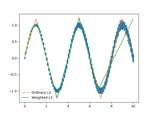
Weighted pwlf fit.

We can see that the weighted pwlf fit tries fit data with low variance better than data with high variance, however the ordinary pwlf fits the data assuming a uniform variance.

reproducible results

The fit and fitfast methods are stochastic and may not give the same result every time the program is run. To have reproducible results you can manually specify a numpy.random.seed on init. Now everytime the following program is run, the results of the fit(2) should be the same.

# initialize piecewise linear fit with a random seed
my_pwlf = pwlf.PiecewiseLinFit(x, y, seed=123)

# Now the fit() method will be reproducible
my_pwlf.fit(2)