Least Squares Sphere Fit

September 13, 2015

Update: 2020-09-20 If you are interested in fitting ellipsoids or formulating other least squares problems check out this new post.

Update: 2018-04-22 I’ve uploaded the data and a demo Python file here.

Update: 2016-01-22 I have added the code I used to make the plot of the 3D data and sphere!

It may not be intuitive to fit a sphere to three dimensional data points using the least squares method. This post demonstrates how the equation of a sphere can be rearranged to formulate the least squares problem. A Python function, which determines the sphere of best fit, is then presented.

So let’s say you have a three dimensional data set. The data points plotted in three dimensional space resemble a sphere, so you’d like to know the sphere that would fit your data set the best. Well I have a sample data set that is well suited for a spherical fit using the least squares method. A plot of data points in three dimensional space can be seen in the following image. Now let’s go through the process fitting a sphere to this data set.

Data points in three dimensions

The general equation of a sphere in $ x $, $ y $, and $ z $ coordinates can be seen below. The center point of the sphere with radius $ r $ is found at the point ( $ x_{0} $, $ y_0 $, $ z_0 $ ). We must rearrange the terms of the equation in order to use the least squares method.

$$ (x - x_0)^2 + (y - y_0)^2 + (z - z_0)^2 = r^2 $$

After expanding and rearranging the terms, the new equation of a sphere is expressed below. This equation can now be expressed in vector/matrix notation.

$$ x^2 + y^2 + z^2 = 2xx_0 + 2yy_0 + 2zz_0 + r^2 - x_0^2 - y_0^2 - z_0^2 $$

The $ \vec{f} $ vector, the $ A $ matrix, and the $ \vec{c} $ vector represents the consolidated terms of the expanded sphere equation. The terms $ x_{i} $, $ y_i $, and $ z_i $ represent the first data point, while $ x_n $, $ y_n $, and $ z_n $ represent the last data point in the data set.

$$ \vec{f} = \begin{bmatrix} x_i^2 + y_i^2 + z_i^2 \\ x_{i+1}^2 + y_{i+1}^2 + z_{i+1}^2 \\ \vdots \\ x_{n}^2 + y_{n}^2 + z_{n}^2 \end{bmatrix} $$

$$ A = \begin{bmatrix} 2x_i & 2y_i & 2z_i & 1 \\ 2x_{i+1} & 2y_{i+1} & 2z_{i+1} & 1 \\ \vdots & \vdots & \vdots & \vdots \\ 2x_n & 2y_n & 2z_n & 1 \\ \end{bmatrix} $$

$$ \vec{c} = \begin{bmatrix} x_0 \\ y_0 \\ z_0 \\ r^2 - x_{0}^2 - y_{0}^2 - z_{0}^2 \end{bmatrix} $$

We now have an over-determined system suitable for the least squares method of a spherical fit. The new equation is seen below. The fit determines the best $ \vec{c} $ from the data points. We can then calculate the sphere’s radius using the terms in the $ \vec{c} $.

$$ \vec{f} = A\vec{c} $$

We can use the above equation to define a simple Python function that will fit a sphere to $ x $, $ y $, and $ z $ data points. The Python NumPy library includes a least squares function that is used to determine the best $ \vec{c} $. The function then returns the radius and center coordinates of the sphere.

import numpy as np
#	fit a sphere to X,Y, and Z data points
#	returns the radius and center points of
#	the best fit sphere
def sphereFit(spX,spY,spZ):
    #   Assemble the A matrix
    spX = np.array(spX)
    spY = np.array(spY)
    spZ = np.array(spZ)
    A = np.zeros((len(spX),4))
    A[:,0] = spX*2
    A[:,1] = spY*2
    A[:,2] = spZ*2
    A[:,3] = 1

    #   Assemble the f matrix
    f = np.zeros((len(spX),1))
    f[:,0] = (spX*spX) + (spY*spY) + (spZ*spZ)
    C, residules, rank, singval = np.linalg.lstsq(A,f)

    #   solve for the radius
    t = (C[0]*C[0])+(C[1]*C[1])+(C[2]*C[2])+C[3]
    radius = math.sqrt(t)

    return radius, C[0], C[1], C[2]

We can easily fit a sphere to our original data set using this function. The resulting sphere of best fit plotted with the original data points can be seen in the following image.

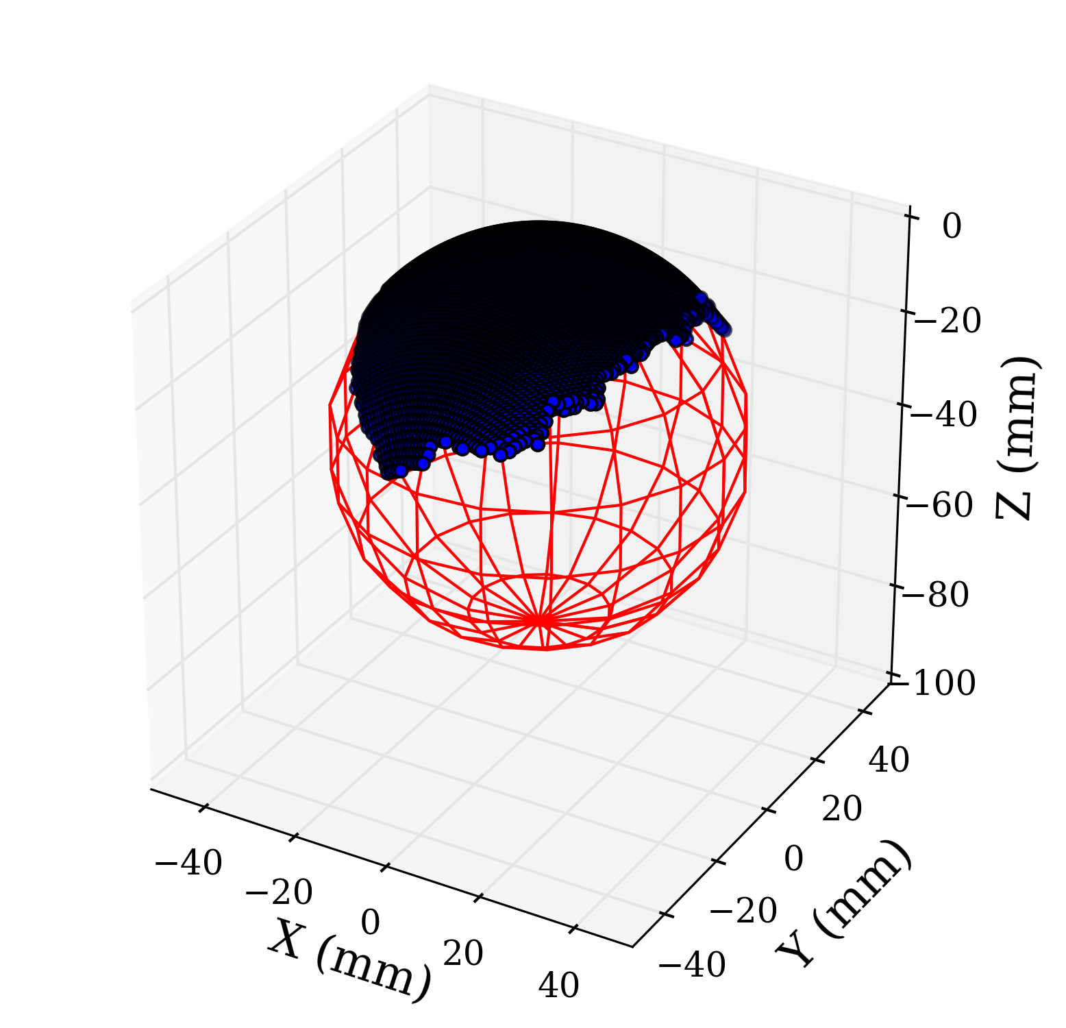
fitted data points in three dimensions

The above 3D plot of the fitted sphere and data was created using the following code.

from matplotlib import rcParams
rcParams['font.family'] = 'serif'
#   3D plot of the
import matplotlib.pyplot as plt
from mpl_toolkits.mplot3d import Axes3D

r, x0, y0, z0 = sphereFit(correctX,correctY,correctZ)
u, v = np.mgrid[0:2*np.pi:20j, 0:np.pi:10j]
x=np.cos(u)*np.sin(v)*r
y=np.sin(u)*np.sin(v)*r
z=np.cos(v)*r
x = x + x0
y = y + y0
z = z + z0

#   3D plot of Sphere
fig = plt.figure()
ax = fig.add_subplot(111, projection='3d')
ax.scatter(correctX, correctY, correctZ, zdir='z', s=20, c='b',rasterized=True)
ax.plot_wireframe(x, y, z, color="r")
ax.set_aspect('equal')
ax.set_xlim3d(-35, 35)
ax.set_ylim3d(-35,35)
ax.set_zlim3d(-70,0)
ax.set_xlabel('$x$ (mm)',fontsize=16)
ax.set_ylabel('\n$y$ (mm)',fontsize=16)
zlabel = ax.set_zlabel('\n$z$ (mm)',fontsize=16)
plt.show()
plt.savefig('steelBallFitted.pdf', format='pdf', dpi=300, bbox_extra_artists=[zlabel], bbox_inches='tight')

Please let me know if you found this post useful!

Please cite this work as:

@book{Jekel2016,
 author = {Jekel, Charles F},
 booktitle = {Obtaining non-linear orthotropic material
              models for pvc-coated polyester via inverse
              bubble inflation},
 chapter = {Appendix A},
 organization = {Stellenbosch University},
 pages = {83--87},
 title = {Digital Image Correlation on Steel Ball},
 url = {https://hdl.handle.net/10019.1/98627},
 year = {2016}
}

Comments