Least Squares Ellipsoid Fit
September 20, 2020
Edit 2021 December 4. In many cases you’ll need to do a non-linear fit to find optimal ellipsoid parameters which I discuss in a newer post as a better way to fit ellipsoids.
In one of my previous posts, I demonstrated how to fit a sphere using the least squares method. In this post I’ll show how you can also fit an ellipsoid using a least squares fit. It ends up being a bit simpler than the sphere. I’ll also include a simple Python example to perform least square ellipsoid fits.
Least-squares method
Mathematical background
The equation of a three dimensional ellipsoid can be described as
where \( x \), \( y \), and \( z \) are the cartesian coordinates of some dataset. Now let’s rearrange the equation to become
where \( \beta_a = 1 / a^2 \), \( \beta_b = 1 / b^2 \), and \( \beta_c = 1/c^2 \). Now we can express the problem in matrix form as the following linear system of equations as
where \( \mathbf{A} \) is a matrix of our squared data components, \( \mathbf{B} \) is a vector of \( \beta \) parameters of the ellipsoid that we intend to solve for, and \( \mathbf{O} \) is a vector of ones. To be explicit we have
for \( n \) number of data points.
Now a least squares problem is a simple optimization which finds the model parameters which minimize the L2 norm between the model and the data. This can be expressed as
and it happens to have a solution of
which is found by setting the first derivative of the linear equation to zero.
Once \( \mathbf{B} \) is solved for, it is only a simple rearrangement to solve for \( a \), \( b \), and \( c \).
Example ellipsoid data
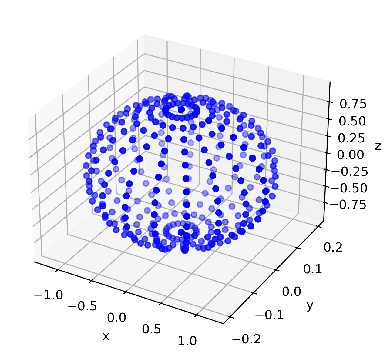
Let’s generate data for an ellipsoid where \( a = 1.2 \), \( b = 0.2 \), and \( c = 0.9 \). This is easiest using parametric equation as
where \( u \in [0, 2\pi] \) and \( v \in [0, \pi] \).
We can quickly generate the cartesian points in Python for this ellipsoid using the following code.
import numpy as np
import matplotlib.pyplot as plt
from mpl_toolkits.mplot3d import Axes3D

a = 1.2
b = 0.2
c = 0.9

u = np.linspace(0., np.pi*2., 20)
v = np.linspace(0., np.pi, 20)
u, v = np.meshgrid(u,v)

x = a*np.cos(u)*np.sin(v)
y = b*np.sin(u)*np.sin(v)
z = c*np.cos(v)

# turn this data into 1d arrays
x = x.flatten()
y = y.flatten()
z = z.flatten()

#   3D plot of ellipsoid
fig = plt.figure()
ax = fig.add_subplot(111, projection='3d')
ax.scatter(x, y, z, zdir='z', s=20, c='b',rasterized=True)
ax.set_xlabel('x')
ax.set_ylabel('y')
ax.set_zlabel('z')
plt.show()
Which gives us the following data and plot in cartesian coordinates.
Python code to fit ellipsoid
Now in order to fit an ellipsoid to the above data, we need to create the matrix \( \mathbf{A} \) and vector \( \mathbf{O} \). Then we’ll use numpy’s least squares solver to find the parameters of the ellipsoid. Lastly we’ll adjust the parameters such that our ellipse is in standard form.
# build our regression matrix
A = np.array([x**2, y**2, z**2]).T

# vector of ones
O = np.ones(len(x))

# least squares solver
B, resids, rank, s = np.linalg.lstsq(A, O)

# solving for a, b, c
a_ls = np.sqrt(1.0/B[0])
b_ls = np.sqrt(1.0/B[1])
c_ls = np.sqrt(1.0/B[2])

print(a_ls, b_ls, c_ls)
Running all of the code together will give you a_ls=1.1999999999999995, b_ls=0.19999999999999993 and c_ls=0.9000000000000006. This is double precision error on our original ellipsoid of \( a = 1.2 \), \( b = 0.2 \), and \( c = 0.9 \). Not too bad! Hopefully you can use this to formulate other least squares problems, or ellipsoids in higher dimensions.
Arbitrary ellipsoids in space
The above least squares problem works well if you data is centered at \( x_0 = 0 \), \( y_0 = 0 \), and \( z_0 = 0 \). Unfortunately, many practical problems will have data that is not centered around the origin. For these cases, we will need to formulate a more expensive non-linear regression problem that uses optimization to find the ellipsoid parameters. We will use jax.numpy as an automatic differentiation code to easily compute derivatives for our custom non-linear regression.
So an arbitrary ellipsoid in 3D space can be defined as
where our ellipsoid parameters are \( x_0 \), \( y_0 \), \( z_0 \), \( a \), \( b \), and \( c \). We can then setup an optimization formulation to find the best six parameters to some arbitrary collection of data in 3D space. Given these six parameters, we can go on to calculate an error between the six parameter ellipsoid and the data set. Optimization will then be used to find the six parameters that minimizes this error.
Given six ellipsoid parameters and any observed data point as \( x_i \), \( y_i \), and \( z_i \), we can predict three separate ellipsoids. This may sound strange at first, but what we are essentially after are three predictions \( \hat{x}_i \), \( \hat{y}_i \), and \( \hat{z}_i \). These predictions are generated by the following equations.