Maximum Likelihood Estimation Linear Regression

October 15, 2016

Edit3 April 17, 2018. I would highly recommend using differential evolution instead of BFGS to perform the optimization. The reason is that the maximum likelihood optimization is likely to have multiple local minima, which may be difficult for the BFGS to overcome without careful use.

Edit2 October 20, 2016. I was passing the integer length of the data set, instead of the floating point length, which messed up the math. I’ve corrected this and updated the code.

Edit October 19, 2016. There was an error in my code, where I took the standard deviation of the true values, when I should have actually been taking the standard deviation of the residual values. I have corrected the post and the files.

I am going to use maximum likelihood estimation (MLE) to fit a linear (polynomial) model to some data points. A simple case is presented to create an understanding of how model parameters can be identified by maximizing the likelihood as opposed to minimizing the sum of the squares (least squares). The likelihood equation is derived for a simple case, and gradient optimization is used to determine the coefficients of a polynomial which maximize the likelihood with the sample. The polynomial that results from maximizing the likelihood should be the same as a polynomial from a least squares fit, if we assume a normal (Gaussian) distribution and that the data is independent and identically distributed. Thus the maximum likelihood parameters will be compared to the least squares parameters. All of the Python code used in this comparison will be available here.

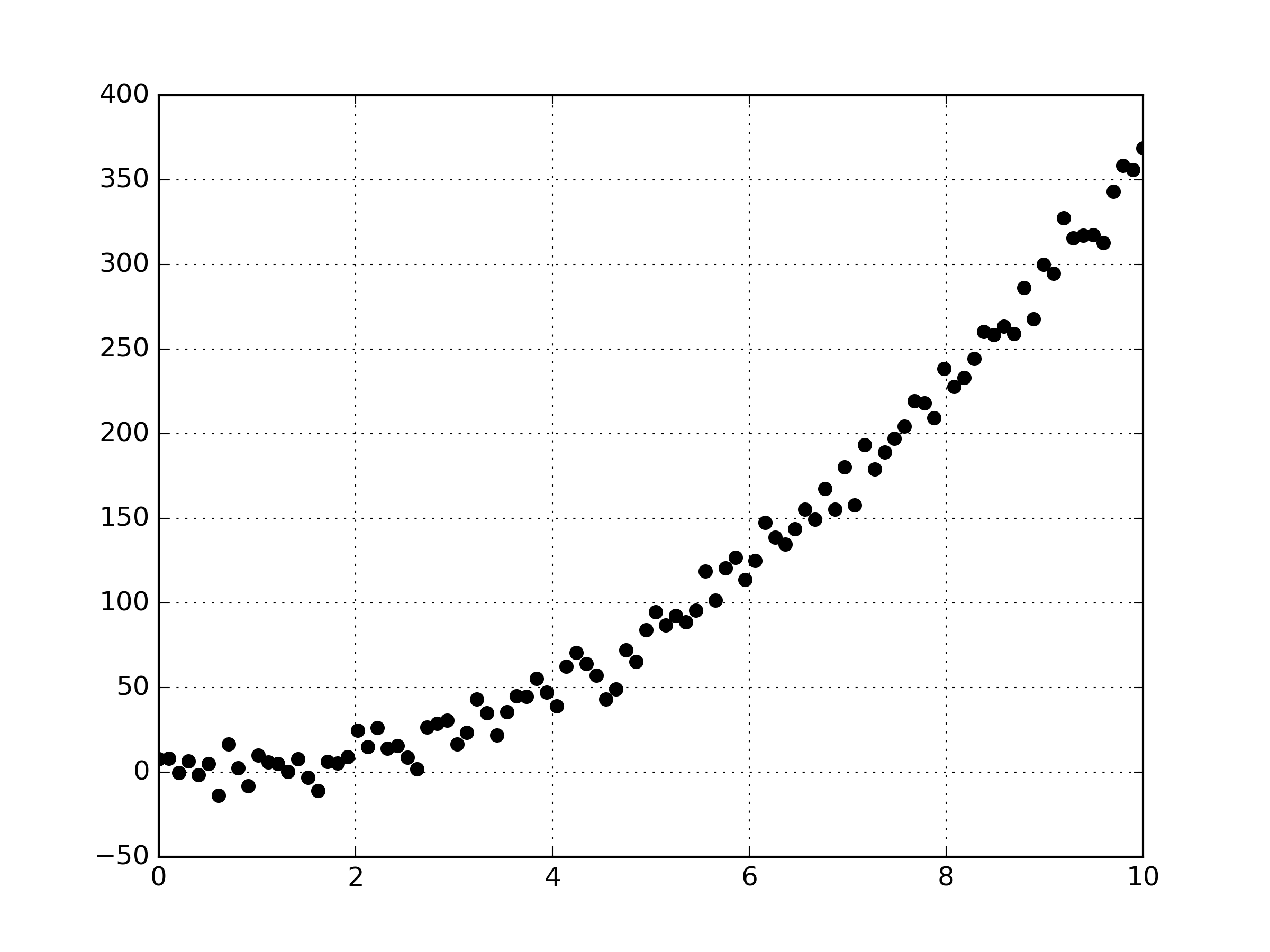
So let’s generate the data points that we’ll be fitting a polynomial to. I assumed the data is from some second order polynomial, of which I added some noise to make the linear regression a bit more interesting.

import numpy as np
x = np.linspace(0.0,10.0, num=100)
a = 4.0
b = -3.5
c = 0.0
y = (a*(x**2)) + (b*x) + c

#   let's add noise to the data
#   np.random.normal(mean, standardDeviation, num)
noise = np.random.normal(0, 10., 100)
y = y+noise

The Python code gives us the following data points.

Image of the polynomial based data points with noise.

Now onto the formulation of the likelihood equation that we’ll use to determine coefficients of a fitted polynomial.

Linear regression is generally of some form

$$ \mathbf{Y} = \mathbf{X}\mathbf{\beta} + \mathbf{r} $$

for a true function $ \mathbf{Y} $, the matrix of independent variables $ \mathbf{X} $, the model coefficients $ \mathbf{\beta} $, and some residual difference between the true data and the model $ \mathbf{r} $. For a second order polynomial, $ \mathbf{X} $ is of the form $ \mathbf{X} = [\mathbf{1}, \mathbf{x}, \mathbf{x^2}]$. We can rewrite the equation of linear regression as

$$ \mathbf{r} = \mathbf{Y} - \mathbf{X}\mathbf{\beta} $$

where the residuals $ \mathbf{r} $ are expressed as the difference between the true model ($ \mathbf{Y} $) and the linear model ($ \mathbf{X}\mathbf{\beta} $). If we assume the data to be of an independent and identically distributed sample, and that the residual $ \mathbf{r} $ is from a normal (Gaussian) distribution, then we’ll get the following probability density function $ f $.

$$ f(x|\mu , \sigma^2) = (2 \pi \sigma^2)^{-\frac{n}{2}} \text{exp}(- \frac{(x-\mu)^2}{2\sigma^2}) $$

The probability density function $ f(x|\mu , \sigma^2) $ is for a point $ x $, with a mean $ \mu $, and standard deviation $ \sigma $. If we substitute the residual into the equation, and assume that the residual will have a mean of zero ($ \mu = 0 $) we get

$$ f(r|0 , \sigma^2) = (2 \pi \sigma^2)^{-\frac{n}{2}} \text{exp}(- \frac{(y - x\beta)^2}{2\sigma^2}) $$

which defines the probability density function for a given point. The likelihood function $ L $ is defined as

$$ L(\beta | x_1, x_2, \cdots, x_n) = \prod_{i=1}^{n}f(x_i | \beta) $$

the multiplication of all probability densities at each $ x_i $ point. When we substitute the probability density function into the definition of the maximum likelihood function, we have the following.

$$ L(\beta | x_1, x_2, \cdots, x_n) = (2 \pi \sigma^2)^{\frac{n}{2}} \text{exp}(- \frac{(\mathbf{Y} - \mathbf{X}\mathbf{\beta})^{\text{T}}(\mathbf{Y} - \mathbf{X}\mathbf{\beta} ) }{2\sigma^2}) $$

It is practical to work with the log-likelihood as opposed to the likelihood equation as the likelihood equation can be nearly zero. In Python we have created a function which returns the log-likelihood value given a set of ‘true’ values ($ \mathbf{Y} $) and a set of ‘guess’ values $ \mathbf{X}\mathbf{\beta} $.

#   define a function to calculate the log likelihood
def calcLogLikelihood(guess, true, n):
    error = true-guess
    sigma = np.std(error)
    f = ((1.0/(2.0*math.pi*sigma*sigma))**(n/2))* \
        np.exp(-1*((np.dot(error.T,error))/(2*sigma*sigma)))
    return np.log(f)

Optimization is used to determine which parameters $ \mathbf{\beta} $ maximize the log-likelihood function. The optimization problem is expressed below.

$$ \{ \hat{\beta}_{\text{MLE}} \} \subseteq \{ \text{arg max} \ln \bigg ( L(\beta | x_1, x_2, \cdots, x_n) \bigg )\} $$

So since our data originates from a second order polynomial, let’s fit a second order polynomial to the data. First we’ll have to define a function which will calculate the log likelihood value of the second order polynomial for three different coefficients (‘var’).

#   define my function which will return the objective function to be minimized
def myFunction(var):
    #   load my  data
    [x, y] = np.load('myData.npy')
    yGuess = (var[2]*(x**2)) + (var[1]*x) + var[0]
    f = calcLogLikelihood(yGuess, y, float(len(yGuess)))
    return (-1*f)

We can then use gradient-based optimization to find which polynomial coefficients maximize the log-likelihood. I used scipy and the BFGS algorithm, but other algorithms and optimization methods should work well for this simple problem. I picked some random variable values to start the optimization. The Python code to run the scipy optimizer is presented in the following lines. Note that maximizing the likelihood is the same as minimizing minus 1 times the likelihood.

#  Let's pick some random starting points for the optimization    
nvar = 3
var = np.zeros(nvar)
var[0] = -15.5
var[1] = 19.5
var[2] = -1.0

#   let's maximize the likelihood (minimize -1*max(likelihood)
from scipy.optimize import minimize
res = minimize(myFunction, var, method='BFGS',
                options={'disp': True})

As it turns out, with the assumptions we have made (Gaussian distribution, independent and identically distributed, $ \mu = 0 $) the result of maximizing the likelihood should be the same as performing a least squares fit. So let’s go ahead and perform a least squares fit to determine the coefficients of a second order polynomial from the data points. This can be done with scikit-learn easily with the following lines of Python code.

#   perform least squares fit using scikitlearn
from sklearn.preprocessing import PolynomialFeatures
from sklearn.linear_model import LinearRegression
from sklearn.pipeline import Pipeline
model = Pipeline([('poly', PolynomialFeatures(degree=2)),
    ('linear', LinearRegression(fit_intercept=False))])

model = model.fit(x[:, np.newaxis], y)
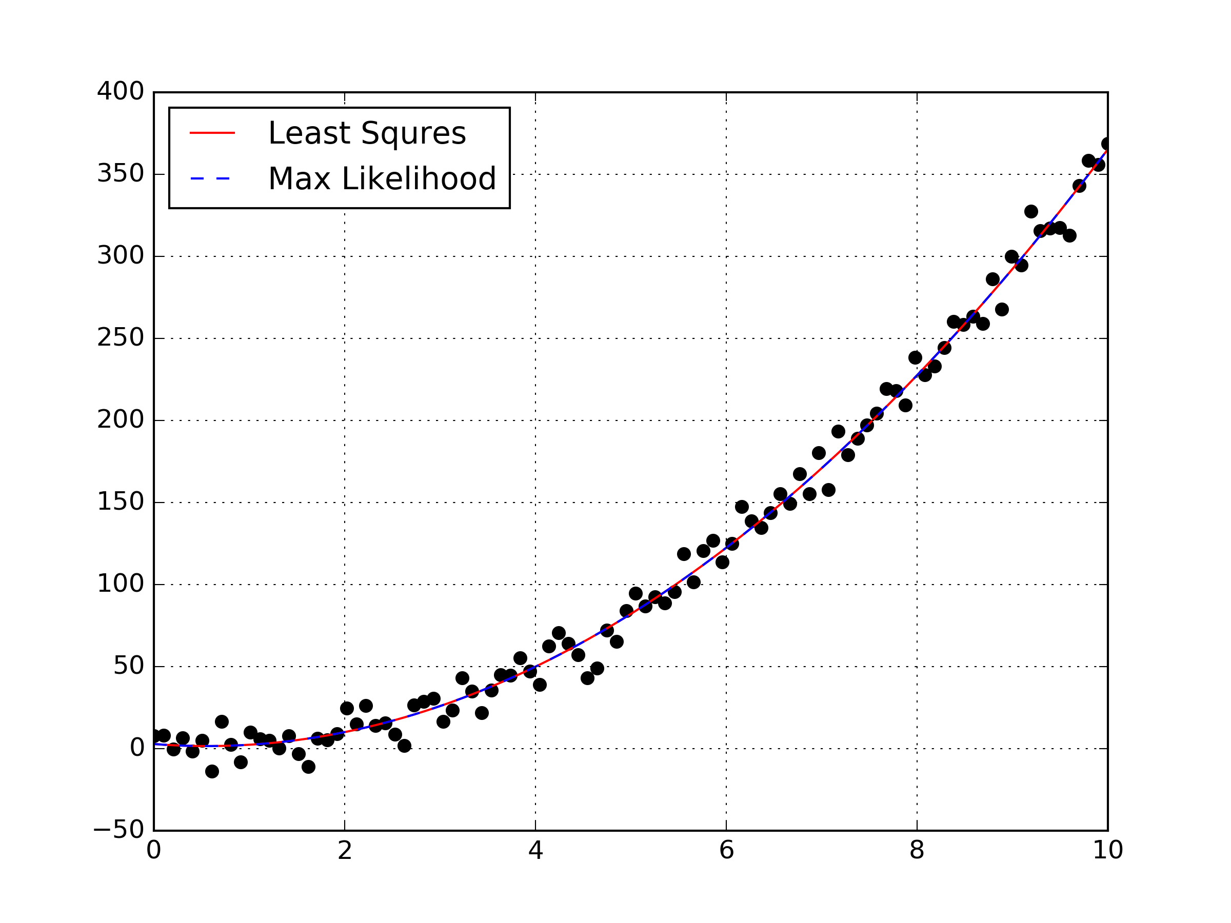
coefs = model.named_steps['linear'].coef_

I’ve made a plot of the data points, the polynomial from maximizing the log-likelihood, and the least squares fit all on the same graph. We can clearly see that maximizing the likelihood was equivalent to performing a least squares fit for this data set. This was intended to be a simple example, as I hope to transition a maximum likelihood estimation to non-linear regression in the future. Obviously this example doesn’t highlight or explain why someone would prefer to use a maximum likelihood estimation, but hopefully in the future I can explain the difference on a sample where the MLE gives a different result than the least squares optimization.

Image of the fitted polynomials and the data points.

A few notes from implementing this simple MLE:

It appears that the MLE performs poorly from bad starting points. I suspect that with a poor starting point it may be beneficial to first run a sum of squares optimization to obtain a starting point of which a MLE can be performed from. Edit October 19, 2016. I re ran optimizations from random starting points by minimizing the root mean square error, and it actually appears that the MLE is a better optimization problem than the RMS error. Edit2 October 26, 2016. This lead to a follow up post here, where I show that actually MLE is a more difficult gradient optimization problem.
I’m not sure about how to select an appropriate probability density function. I’m not sure what the benefit of using MLE over least squares if I always assume Gaussian… I guess I’ll always know the standard deviation, and that the mean may not always be zero.

Comments