There have been a number of people asking how to use pwlf when you don’t know how many line segments to use. I’ve been recommending the use of a regularization technique which penalizes the number of line segments (or model complexity). This is problematic in a few ways:

• It’s an expensive three layer optimization problem (least squares fit, find break point locations, find number of line segments).
• The result will be dependant upon the penalty parameter which is problem specific. Something like cross validation could be used to select the parameter, but again this can be expensive.

A large portion of the expense results from searching for breakpoints on a continuous domain. Once the breakpoint locations are known, then the resulting piecewise continuous model is just a simple least squares fit. In many applications it is reasonable to assume some discrete set of possible breakpoint locations. For instance, it may be reasonable to assume that breakpoints can only occur at the points within the data. This would work well for a large amount of data that is evenly distributed in the domain. Alternatively, one could specify a large number of possible breakpoint locations over the domain. The 0.4.0 version of pwlf will include a function which returns the linear regression matrix, which will be used later on to perform Elastic Net fits to a complex function.

Least Squares Fits

A least squares fit can be used to solve for the model parameters \((\mathbf{\beta}) \) from a discrete list of possible breakpoint locations. Then the value of a model parameter \((|\beta_3|) \) would tell whether a breakpoint was significant. The following example demonstrates this on a simple problem with two distinct line segments.

import numpy as np
import matplotlib.pyplot as plt
import pwlf

x = np.array([1, 2, 3, 4, 5, 6, 7, 8, 9, 10, 11, 12, 13,
              14, 15])
y = np.array([5, 7, 9, 11, 13, 15, 28.92, 42.81, 56.7,
              70.59, 84.47, 98.36, 112.25, 126.14,
              140.03])

# initialize pwlf on data
my_pwlf = pwlf.PiecewiseLinFit(x, y)
# perform a least squares fit with the breakpoints
# occurring at the exact x locations
ssr = my_pwlf.fit_with_breaks(x.copy())

# predict on the domain
xhat = np.linspace(x.min(), x.max(), 100)
yhat = my_pwlf.predict(xhat)

This results on the following fit which appears excellent.

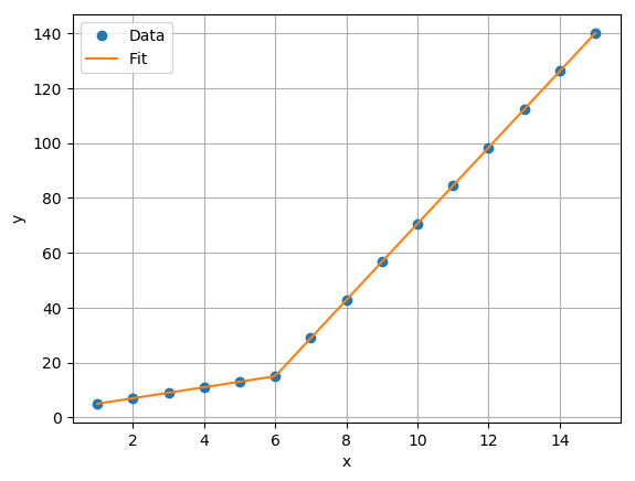
Let’s take a look at the model parameters.

print(my_pwlf.beta)

[ 5.00000000e+00  2.00000000e+00 -8.72635297e-14
  4.06341627e-14 -1.99840144e-15 -6.66133815e-16
  1.19200000e+01 -3.00000000e-02 -1.24344979e-14
  1.29896094e-14 -1.00000000e-02  1.00000000e-02
  2.06085149e-14 -5.27564104e-14  7.40345285e-14]

The first parameter is the model offset and the second parameter is the slope of the first line. The remaining parameters are related to the slopes of subsequent lines. The small and near zero parameters imply that the slope didn’t change from the previous breakpoint. We can see that seventh parameter is significant, and it so happens that it corresponds to the seventh data point. This is the first data point on the second line!

There are a few obvious problems with this method. One problem is that the least squares problem becomes ill-posed in the case when you have more unknowns than data points. Additionally, this method is likely to result in a poor model that overfits the data. The following example follows the previous procedure to fit a continuous piecewise linear model to a noisy sine wave.

# select random seed for reproducibility
np.random.seed(123)
# generate sin wave data
x = np.linspace(0, 10, num=100)
y = np.sin(x * np.pi / 2)
ytrue = y.copy()
# add noise to the data
y = np.random.normal(0, 0.05, 100) + ytrue

# initialize pwlf on data
my_pwlf = pwlf.PiecewiseLinFit(x, y)
# perform a least squares fit with the breakpoints
# occuring at the exact x locaitons
ssr = my_pwlf.fit_with_breaks(x.copy())

# predict on the domain
xhat = np.linspace(x.min(), x.max(), 1000)
yhat = my_pwlf.predict(xhat)

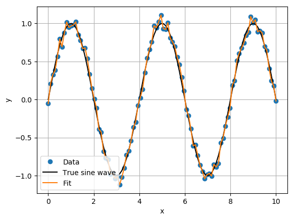
The result was a continuous piecewise linear function that has overfit the data. You’ll find that most of the \((\mathbf{\beta}) \) parameters are active, with an average absolute value of 1.1.

Elastic Net for noisy data

We can use a linear model regularizer such as Elastic Net to prevent this overfitting. The least squares problem minimizes

which is prone to overfitting when there are a lot of possible \((\mathbf{\beta}) \) parameters. The Elastic Net uses both L1 (LASSO) and L2 (Ridge regression) to penalize the model complexity. This prevents overfitting. The objective function of the Elastic Net is to minimize

for some \((\lambda_1, \lambda_2) \) penalty parameters. The Elastic Net solution stats each \((\mathbf{\beta}) \) parameter at zero, and slowly activates a parameter one at a time through the iterations until convergence. This work well for continuous piecewise linear functions, where a zero parameter value corresponds to that breakpoint being inactive.

Scikit-learn has implemented the Elastic Net regularizer in ElasticNet. The important penalty parameters to select will be l1_ratio and alpha. However, we’ll use ElasticNetCV which will select these parameters based on cross validation results. The following example perform the Elastic Net fit to the noisy sine wave.

from sklearn.linear_model import ElasticNetCV
my_pwlf_en = pwlf.PiecewiseLinFit(x, y)
# copy the x data to use as break points
breaks = my_pwlf_en.x_data.copy()
# new in 0.4.0; creates the linear regression matrix A 
A = my_pwlf_en.assemble_regression_matrix(breaks, my_pwlf_en.x_data)

# set up the elastic net
en_model = ElasticNetCV(cv=5,
                        l1_ratio=[.1, .5, .7, .9,
                                  .95, .99, 1],
                        fit_intercept=False,
                        max_iter=1000000, n_jobs=-1)
# fit the model using the elastic net
en_model.fit(A, my_pwlf_en.y_data)

# predict from the elastic net parameters
xhat = np.linspace(x.min(), x.max(), 1000)
yhat_en = my_pwlf_en.predict(xhat, breaks=breaks,
                             beta=en_model.coef_)

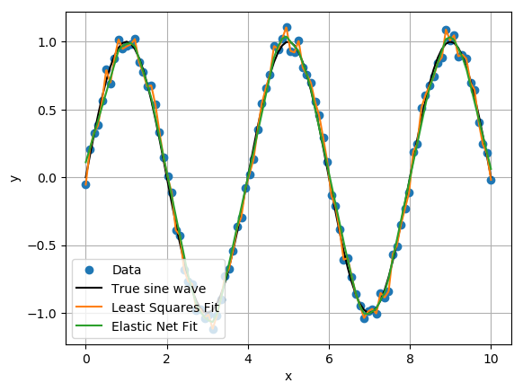
We can see the Elastic Net results are a much better fit to the sine wave than the least squares fit. In fact, the fit appears to resemble a result from support vector regression!

Perhaps we can use the Elastic Net fit to identify important breakpoint locations. Again, the first two parameters are related to the first line segment, so we’ll always want to grab the first two parameters. However, after the first two parameters we’ll only grab parameters that have an absolute value larger than a threshold. The rational for this is that when \((\mathbf{\beta}) \) parameters are small the breakpoint become inactive (effectively removing a column from the regression matrix).

true_list = np.zeros(breaks.size, dtype=bool)
true_list[:2] = True
for i in range(breaks.size):
    if np.abs(en_model.coef_[i]) > 2e-1:
        true_list[i] = True
    else:
        true_list[i] = False
# new list of important breakpoint locations
new_breaks = breaks[true_list]
n_segments = new_breaks.size - 1.

# get the y value from these new breakpoints form the EN model
ybreaks = my_pwlf_en.predict(new_breaks)

# fit a least squares model from these new breakpoints
ssr = my_pwlf.fit_with_breaks(new_breaks)
yhat = my_pwlf.predict(xhat)

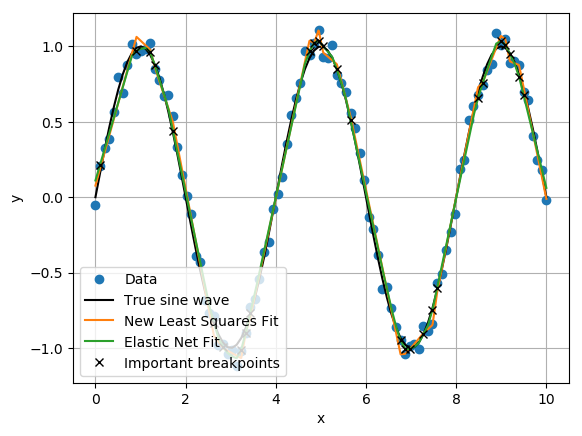
If we filter the breakpoints with the above code, we’ll have 28 line segments and the following important breakpoints. Unfortunately, the new least squares fit at these new breakpoint locations still overfits the true function.

Conclusion

A couple alternative strategies are presented to find the number of line segments instead of running an expensive three-layer optimization. If you do not have much noise in your data, you can try to perform a least squares fit where the breakpoints occur at the data points. Alternatively, if you have noise in your data you can use something like the Elastic Net regularizer to perform the fit. (I have a paper on approximating the noise in 1D data.) After the fits are performed, you can analyze the model parameters (or slopes) to identify unique line segments in your model. A small \(\beta \) parameter implies that the breakpoint is not active.